Importance Sampling - Clearly Explained
Importance Sampling is a tool that helps us tackle a common challenge: calculating expectations. While that might sound like a straightforward task, it often becomes a formidable problem, especially when dealing with high-dimensional data. In this blog post, we’ll delve into the intricacies of this technique and explore its significance.
- The Importance of Calculating Expectations
- Monte Carlo Methods for Approximating Expectations
- Properties of Monte Carlo Estimates
- Introduction to Importance Sampling
- Example of Importance Sampling
- The Benefits of Importance Sampling
- Considerations and Challenges
- Final Thoughts
The Importance of Calculating Expectations
Expectations, in this context, refer to a way of summarizing complex information about a random variable. They are essentially the answers that many of our machine learning algorithms are seeking.
Imagine we have a continuous random variable, let’s call it $x$ (x can be a vector), and we want to understand something about it. We’re not just interested in one specific value of $x$, but rather, we want to capture its entire distribution and use that to compute certain quantities of interest.
Mathematically, this means we want to calculate the expectation of a function $f(x)$ with respect to the probability density function $p(x)$, where:
-
$x$ is the random variable.
-
$f(x)$ is a scalar function that we’re interested in, which could represent anything from model predictions to real-world measurements.
-
$p(x)$ is the probability density function that describes the likelihood of different values of $x$ occurring.
Now, this might seem a bit abstract, so let’s break it down. Think of the expectation as a probability-weighted average of the function $f(x)$ over the entire space where $x$ can exist. In a way, it’s like trying to find the “typical” value of $f(x)$ based on how likely different values of $x$ are.
To represent this mathematically, we often use the following notation:
$E[f(x)] = \int f(x) p(x) dx$
In this formula, the integral symbol (∫) represents a kind of super-sum over all possible values of $x$, and dx is an infinitesimally small step as we sweep through those values.
Now, this might seem straightforward when dealing with simple, low-dimensional problems. However, we often encounter situations where calculating this expectation exactly becomes an intractable task. Why? Because the dimension of $x$ can be incredibly high, leading to an exponentially vast space of possibilities. This is where the challenge arises: how can we compute this expectation when it’s impossible to calculate the integral directly?
The answer to this conundrum lies in a powerful technique known as Monte Carlo methods, and at the heart of Monte Carlo methods is the idea of approximation through random sampling. In the next section, we’ll delve deeper into these methods and how they help us tackle the formidable task of calculating expectations.
Monte Carlo Methods for Approximating Expectations
Monte Carlo methods are a class of statistical techniques that provide a clever way to approximate expectations without having to perform infeasible calculations. Instead of trying to calculate the expectation directly, these methods rely on the power of random sampling to provide estimates. Here’s how they work:
Imagine you have a function $f(x)$ and a probability density function $p(x)$, and you want to calculate the expectation $E[f(x)] = \int f(x)p(x) dx$. As mentioned earlier, this integral can be incredibly challenging to compute directly, especially in high-dimensional spaces. But what if we could estimate it using random samples?
The core idea behind Monte Carlo methods is simple: rather than calculating the expectation as an integral, we approximate it with an average. Here’s how it works:
-
We collect $n$ random samples of $x$ from the distribution described by $p(x)$.
-
For each of these samples, we evaluate the function $f(x)$.
-
We then take the average of all these $f(x)$ values.
Mathematically, this approximation can be written as:
$s = \frac{1}{n} \sum_{i=1}^{n} f(x_i)$
Where:
-
$s$ is our estimate of the expectation.
-
$n$ is the number of samples we collect.
-
$x_i$ are the random samples drawn from the distribution $p(x)$.
The magic of Monte Carlo methods lies in the fact that as the number of samples $n$ gets larger, our estimate $s$ approaches the true expectation $E[f(x)]$. In other words, by repeatedly sampling from $p(x)$ and averaging the results, we converge to the correct answer.
Properties of Monte Carlo Estimates
Now that we understand the basic premise of Monte Carlo methods for approximating expectations, it’s important to dive deeper into the properties that support these estimations. Two key concepts to explore are bias and variance, which play a crucial role in determining the reliability and accuracy of Monte Carlo estimates.
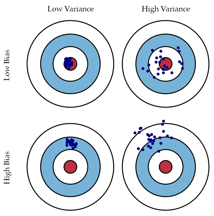 Bias vs. Variance (source)
Bias in Monte Carlo Estimates
In statistics, bias refers to the tendency of an estimator to consistently overestimate or underestimate a parameter. In the context of Monte Carlo estimation, it’s essential to know whether our estimates tend to systematically deviate from the true expectation. The good news is that Monte Carlo estimates are unbiased.
What does this mean? It means that if we were to repeat the Monte Carlo estimation process many times, each time with a different set of random samples, the average of those estimates would converge to the true expectation we are trying to calculate. In other words, the average of our estimates does not consistently overestimate or underestimate the true value; it approaches it as the number of samples increases.
This property is particularly valuable because it ensures that, on average, our Monte Carlo estimates are reliable and not systematically skewed in one direction.
Variance in Monte Carlo Estimates
While bias tells us whether our estimates tend to be on target, variance provides insight into how much our estimates fluctuate around that target. In simple terms, it measures the spread or dispersion of our estimates. In the context of Monte Carlo methods, we are interested in understanding how much individual estimates can deviate from the average estimate.
The variance of a Monte Carlo estimate depends on two main factors:
-
The variance of the function $f(x)$: If $f(x)$ has high variance, meaning it varies significantly across different values of $x$, then our estimates are likely to be more spread out and less precise.
-
The number of samples $n$: As we increase the number of samples, the variance tends to decrease. In other words, with more samples, our estimates become more stable and less sensitive to random fluctuations in the data.
It’s important to note that while the bias of Monte Carlo estimates remains consistently low, the variance decreases as we collect more samples. This means that, in practice, we can improve the accuracy of our Monte Carlo estimations by simply increasing the sample size.
The Central Limit Theorem
One fascinating aspect of Monte Carlo estimates is their convergence behavior, which is heavily influenced by the Central Limit Theorem. This theorem tells us that as the number of samples $n$ becomes large, the distribution of our Monte Carlo estimates approaches a normal distribution.
In simple terms, it means that regardless of the specific distributions $p(x)$ and $f(x)$, as long as we have a sufficiently large number of samples, the distribution of our estimates will resemble a bell curve, with the mean of the estimates converging to the true expectation we seek to calculate.
This property is incredibly valuable because it allows us to make statistical inferences about our Monte Carlo estimates. We can compute confidence intervals, assess the precision of our estimates, and better understand the inherent uncertainty associated with our calculations.
In the next section, we’ll introduce the concept of importance sampling, which is a technique that builds upon Monte Carlo methods to further improve the efficiency of estimating expectations. We’ll explore how importance sampling can help us choose the right samples and distributions to reduce variance and enhance the accuracy of our estimations.
Introduction to Importance Sampling
Having grasped the fundamentals of Monte Carlo methods for estimating expectations, it’s time to embark on the journey of enhancing these estimations through a powerful technique known as importance sampling. Importance sampling is a valuable tool in our toolkit, especially when we need to make our Monte Carlo estimates even more efficient and accurate.
The Motivation for Importance Sampling
Before we dive into the intricacies of importance sampling, let’s first understand why it’s needed. In Monte Carlo estimation, we often encounter scenarios where the distribution $p(x)$ is challenging to sample from or where it’s simply not the most efficient choice for our estimation task.
Consider the expectation we want to calculate, denoted as $E[f(x)] = \int f(x) p(x) dx$. If $p(x)$ is a complex or high-dimensional distribution, obtaining random samples from it can be computationally expensive or even impossible. This is especially true when dealing with real-world datasets or intricate models.
Here’s where importance sampling steps in. It offers a solution by introducing a new distribution, $q(x)$, which we get to choose. This distribution, when selected wisely, can make the process of estimating expectations significantly more efficient and accurate.
The Trick Behind Importance Sampling
Now, let’s uncover the core trick behind importance sampling. At its essence, importance sampling involves a simple mathematical maneuver. We take the integrand $\int f(x)p(x)$ and multiply it by the ratio of $q(x)$ over itself, which is essentially just multiplying by 1. Here’s what it looks like:
$E[f(x)] = \int f(x) \frac{p(x)}{q(x)} q(x) dx$
This may seem like a meaningless change, but it has interesting implications. By multiplying and dividing by $q(x)$, we’re essentially saying, “Let’s consider the probability-weighted average of a new function, where the probability is given by $q(x)$ instead of $p(x)$.”
We can rewrite this as:
$E[f(x)] = \int \left(\frac{p(x)}{q(x)} \cdot f(x)\right) q(x) dx$
This clever manipulation allows us to rewrite the original expectation in terms of a new function that depends on both $p(x)$ and $q(x)$. Now, here’s the key: we can estimate this new expectation using samples drawn from $q(x)$.
The Power of Importance Sampling
By choosing $q(x)$ strategically, we can tap into the power of importance sampling to enhance our estimation process. The resulting estimate, which we’ll denote as $r$, is calculated as follows:
$r = \frac{1}{n} \sum_{i=1}^{n} \left(\frac{p(x_i)}{q(x_i)} f(x_i)\right)$
Where:
-
$n$ is the number of samples drawn from $q(x)$.
-
$x$i are the random samples drawn from $q(x)$.
Now, what makes importance sampling particularly valuable? First, it shares a critical property with plain Monte Carlo estimation: it’s unbiased. This means that, on average, our importance sampling estimate $r$ will converge to the true expectation $E[f(x)]$ as the number of samples increases.
Second, and perhaps even more exciting, importance sampling can often lead to a reduction in variance compared to plain Monte Carlo. In other words, our estimates become less scattered and more precise. This variance reduction is achieved by wisely choosing $q(x)$ so that it focuses sampling on regions where the absolute value of p(x)f(x) is high.
In the next section, we’ll delve into practical examples to demonstrate how importance sampling can significantly improve the accuracy of our estimations, especially in scenarios where the original distribution $p(x)$ poses challenges. We’ll also explore considerations and challenges when selecting $q(x)$ in practice.
Example of Importance Sampling
To truly grasp the power of importance sampling, let’s delve into a practical example where it can make a substantial difference in the accuracy of our Monte Carlo estimates. In particular, we’ll explore a scenario where the use of importance sampling can significantly reduce variance, leading to more reliable and efficient estimations.
The Problem Setup
Imagine we have a probability density function $p(x)$ and a function $f(x)$ that we want to calculate the expectation for. For this example, we’ll use a specific $p(x)$ and $f(x)$:
-
$p(x)$ represents the probability density function, which describes how likely different values of $x$ are.
-
$f(x)$ is the function we want to calculate the expectation of.
Let’s visualize this scenario by plotting $p(x)$ and $f(x)$. For the sake of simplicity, we’ll use a one-dimensional example:
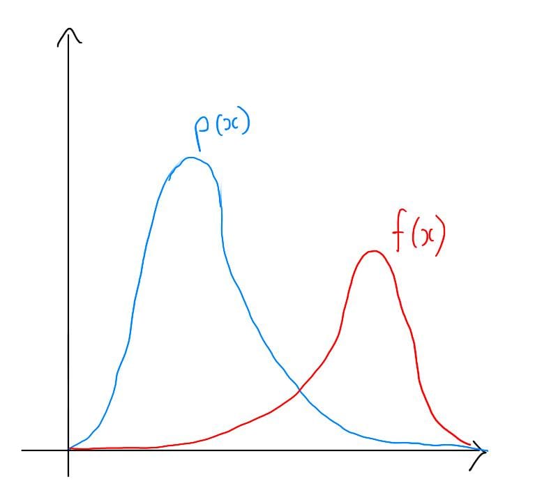 Plots of p(x) and f(x)
In this example, $f(x)$ has high values only in rare events under the distribution $p(x)$. These rare events, while important, make it challenging to estimate the expectation accurately because most random samples drawn from $p(x)$ will not contribute much to the average. As a result, our Monte Carlo estimates can exhibit high variance, meaning they can vary significantly from one estimation to another.
Using Importance Sampling
Now, let’s see how importance sampling can come to the rescue. The key idea is to introduce a new distribution $q(x)$ that guides our sampling process to focus on regions where the absolute value of $p(x)f(x)$ is high.
In this example, let’s choose $q(x)$ to be a distribution that closely approximates $p(x)$ in most regions but places more probability density where $f(x)$ has high values. By doing so, we’re essentially making our samples “smarter” by directing them toward the more critical areas.
Here’s a visualization of $q(x)$ alongside $p(x)$ and $f(x)$:
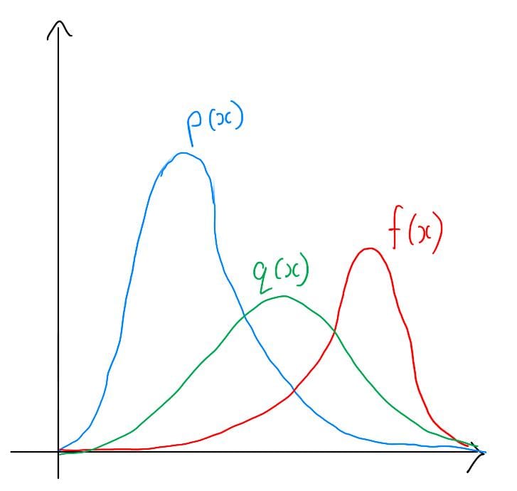 Plots of p(x), f(x), and q(x)
With $q(x)$ in place, we can now calculate the new expectation using importance sampling.
The Benefits of Importance Sampling
The magic happens when we compare the estimates obtained using plain Monte Carlo and importance sampling. What we typically observe is a significant reduction in the variance of our estimates when importance sampling is employed.
In general, the estimates obtained through importance sampling exhibit much less variation compared to those obtained through plain Monte Carlo. This means that with importance sampling, we have a more stable and precise estimate of the expectation, even in scenarios where $f(x)$ has high values in rare events.
Considerations and Challenges
While importance sampling is a powerful technique, it’s essential to recognize that selecting the right $q(x)$ distribution can be challenging, especially in high-dimensional spaces. An inappropriate choice of $q(x)$ can lead to a wildly varying density ratio $p(x)/q(x)$ across samples, resulting in a high variance in our estimates.
In practice, finding the ideal $q(x)$ often involves domain knowledge and experimentation. We may choose $q(x)$ based on our understanding of the problem or simply opt for a distribution that approximates $p(x)$ well in most regions.
Final Thoughts
Importance sampling is a valuable tool that can significantly improve the efficiency and accuracy of Monte Carlo estimates, especially in scenarios where the original distribution $p(x)$ presents challenges. By selecting $q(x)$ strategically, we can guide our samples to focus on the most important regions, leading to more reliable estimations with reduced variance. However, the art of choosing $q(x)$ wisely remains a key consideration in practice.
If you would like to check out more of the AI Math-related content, feel free to check out the AI Math page of this site.