NT-Xent Loss - A Quick Overview
The Normalized Temperature-scaled Cross Entropy loss (NT-Xent loss), a.k.a. the “multi-class N-pair loss”, is a type of loss function, used for metric learning and self-supervised learning. Kihyuk Sohn first introduced it in his paper “Improved Deep Metric Learning with Multi-class N-pair Loss Objective”. It was later popularized by its appearance in the “SimCLR” paper by the more commonly used term “NT-Xent”.
In this article, I will cover the following points:
-
NT-Xent Loss Definition
-
High-level Overview
-
Deeper Dive
-
Pseudocode
-
Implementation
NT-Xent Loss Definition
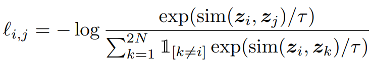 Eq 1: NT-Xent loss as given in the SimCLR paper
Despite the intimidating look at a glance, the equation is fairly simple. The NT-Xent loss denotes the loss that is observed for a pair of samples i and j.
To understand what’s happening here, let’s first get a high-level understanding of what the equation is giving us. This will be followed by a section going into a bit more detail.
A High-Level Overview of NT-Xent
Let’s look at the fraction. The fraction as a whole may seem familiar to those who’ve come across the softmax activation function. The difference is that, instead of getting the ratio of the exponentials of each output node against the other output nodes (as in softmax), in this case, we’re exponentiating the similarities between two output vectors against the similarities between one output vector, and every other output vector. Thus, a high similarity between i and j would result in the fraction taking a higher value compared to pairs with lower similarity.
However, what we need is the opposite of this. We need pairs with higher similarities to give a lower loss. To achieve this, the result is negated.
The next question you may have is, “Why do we need the log term?”.
-
For one thing, it ensures that the loss we get is positive. The fraction is always less than one and the log value of a number less than one is negative. This, along with the negation mentioned earlier, results in a positive loss.
-
The other thing is that you can think of it as something to counteract the possibility of very large exponentials causing very small fractions. Changes in very small values may not be too noticeable to the network, and thus, scaling using
logis bound to be favorable. -
And the final reason is,
 It just works
A Deeper Dive
Cosine Similarity
sim gives us the (cosine) similarity between the vectors zᵢ and zⱼ. These vectors are usually the output of some neural network. To put it simply, the smaller the element-wise difference between the two vectors, the higher the resulting value.
Another thing to note in the below equation (Eq 2) is that, because we divide by the magnitudes of the two vectors, the cosine similarity can be considered as an L2 Normalization. Empirically, this, along with the temperature (τ), has been shown by the SimCLR paper to lead to significant improvements in contrastive accuracy.
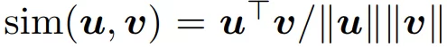 Eq 2: Cosine similarity
Temperature
The value of this similarity is divided by a value denoted by τ (tau), a.k.a. the temperature. τ is used to control the influence of similar vs dissimilar pairs. The lesser τ is relative to 1, the greater the difference in the value of the term exp(sim(zᵢ, zⱼ)/τ) for similar pairs vs that for a dissimilar pair.
The Summation
Let’s pay our attention to the denominator.
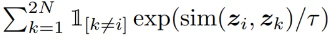 The denominator of the NT-Xent loss
As previously mentioned, the NT-Xent loss is applied to pairs of samples. In the case of SimCLR, each pair is obtained by augmenting a single image. Therefore, each sample has one positive sample and 2(N - 1) negative samples. Consequently, to loop over all possible outcomes, we loop from k=1 to k=2N, and simply avoid the case where both k and i are referring to the same image. This is achieved using the following term.
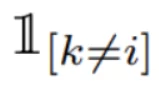 1 if k is not equal to i, else 0
Pseudocode
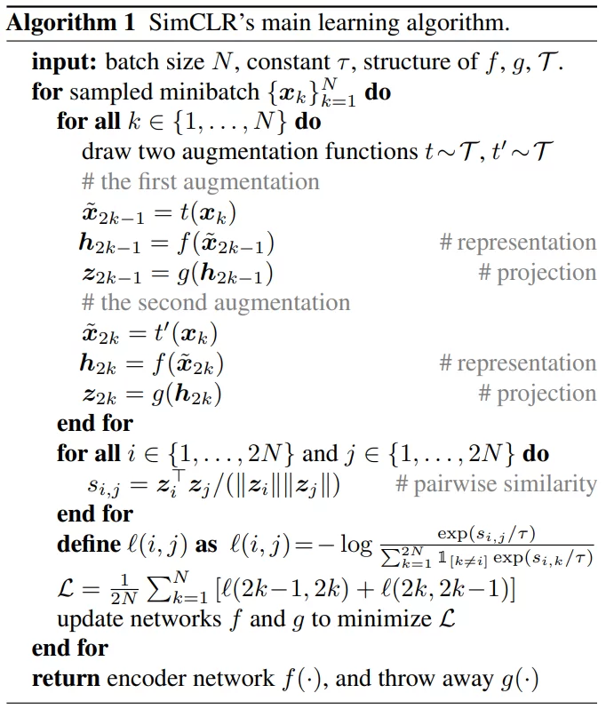 SimCLR pseudocode
The above pseudocode is that of the SimCLR algorithm. However, it gives a good idea as to how one might approach the implementation of the loss.
Of the steps shown in the image, the lines that concern the NT-Xent loss can be summarized as follows:
-
For each minibatch (a batch of N samples), generate a pair of augmented samples (positive pair) and calculate the output z value.
-
For every possible pair in the 2N samples that were generated, calculate the pairwise cosine similarity.
-
For every possible pair in the 2N samples that were generated, calculate the loss.
Implementation of NT-Xent Loss
In the case of most deep learning frameworks, the implementations of the NT-Xent loss are readily available on the internet. For example, PyTorch Metric Learning offers a great implementation of the NT-Xent loss for PyTorch, available here. Similarly, one can find implementations for Tensorflow here or here.
Final Thoughts
The NT-Xent loss is gaining more and more traction with the progression of self-supervised learning and other applications of contrastive learning. As a result, it has become essential to have a good understanding of how and why it works, in order to apply it to its strengths. If you’re interested in seeing my other AI Math-related content, feel free to head over to the AI Math section of the blog.