Kalman Filters - A Quick Introduction
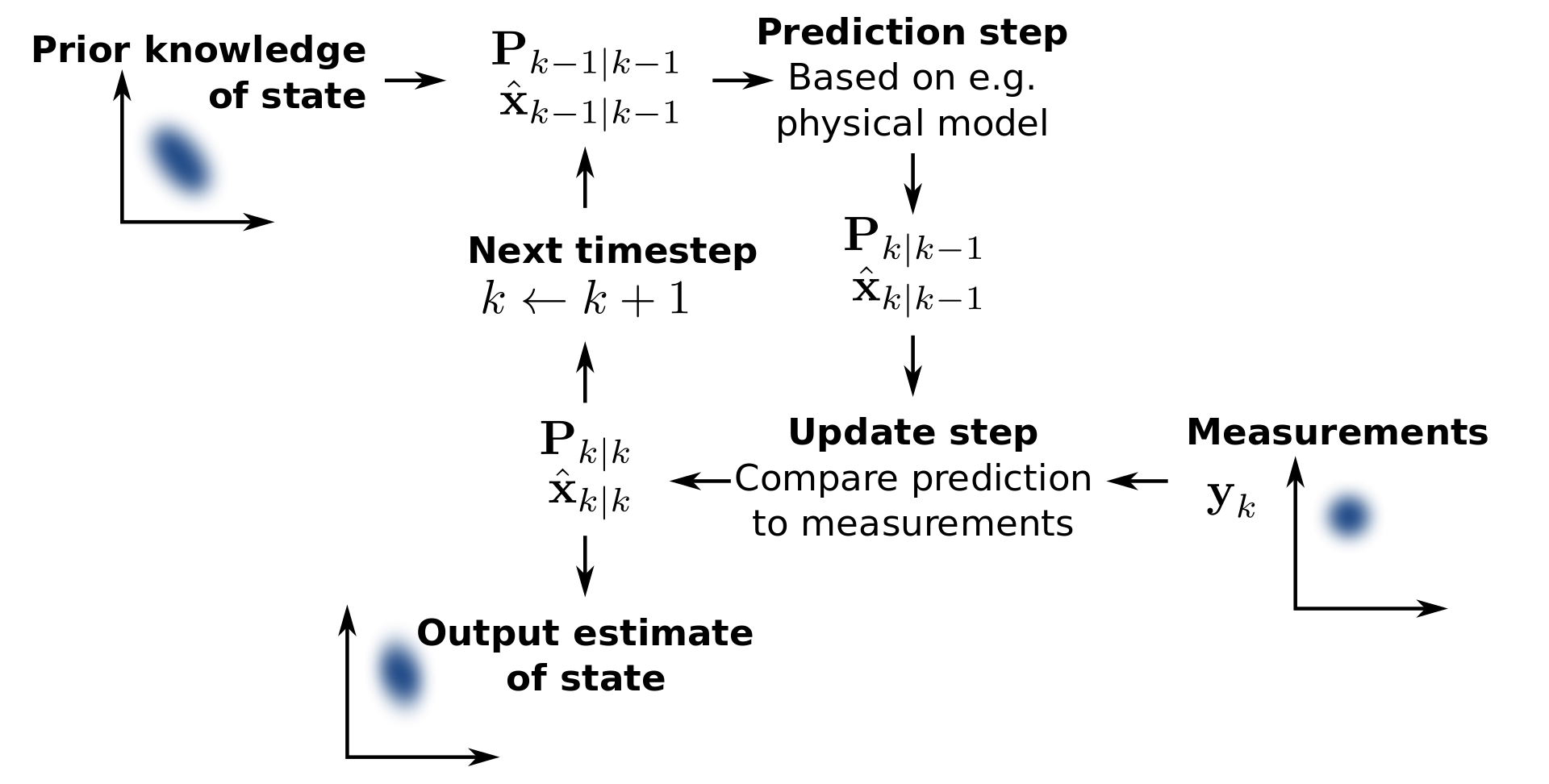 The Kalman Filtering Process
In this blog post, we’ll be discussing Kalman filters, a commonly used technique for estimating the state of a system in a dynamic environment by integrating sensor measurements and predictions.
Let me introduce the utility of Kalman filters with an example.
Imagine a car traveling on a straight road. The car is traveling at a constant speed and is integrated with GPS sensors. Say the car’s location at time $0$ is $x_0$ and its speed is $v$.
Given this information, how would we go about calculating the location of the car at time $t$? In a perfect world, this would be simply:
So, in a perfect world, we wouldn’t really need GPS. We can just calculate where we are at a given time using some equations.
In reality, however, this is often not the case. The car is traveling against factors like air resistance, friction, bumps in the road, etc. Further, the measurements of GPS sensors are rarely perfect. So, we can’t rely on either of them individually. However, they both carry information that may be useful to come up with a more accurate answer. But how do we combine this information? That’s where Kalman filters come in.
Steps to Kalman Filtering
There are two main steps to Kalman filtering:
- Prediction Step
- Correction/Update Step
Let’s go back to our car example.
1. Prediction Step
Remember how we came up with an equation for $x_t$ assuming ideal conditions? This is the prediction step.
We use the control commands (in our example, this would be the command to go at a constant speed of $v$ for a time $t$) to estimate the current state of the system (in our example, this would be the distance $x_t$ moved by the car).
2. Correction/Update Step
Next, say we take a measurement from the GPS sensor at time $t$ (say $m_t$) and we observe that it estimates a slightly different location than what we got with $x_t$.
Now comes the slightly tricky part. We need to combine $x_t$ and $m_t$. Sure, we can get the average of the two, but is that really the best result that we can get? What if we’re more confident about the value $x_t$ than $m_t$ (or vice versa)? In such a case, taking the average may not be the best result.
For these cases, we calculate something called the Kalman ratio ($K$) as follows:
where $\sigma_x$ is the variance of the prediction and $\sigma_m$ is the variance of the measurement.
You can think of the variance as a measure of how much a certain value may vary. In other words, it’s a measure of how uncertain we’re about the value of a given variable.
Let’s try to understand the behavior of the above equation. When we are completely certain about our prediction (i.e., $\sigma_x=0$), $K=0$. On the other hand, when we are completely certain about our GPS measurement (i.e., $\sigma_m=0$), $K=1$.
Therefore, we can arrive at the following equation for our corrected prediction:
The Kalman ratio $K$ is a value between $0$ and $1$. When the value is $1$, $x_t^+ = m_t$ and when the value is $0$, $x_t^+ = x_t$.
Slightly Deeper into the Math
The above explanation is a simplified version of the actual math behind Kalman filters in order to get an intuitive understanding. In this section, let’s discuss the math in a bit more detail.
First, we can generalize our $x_t$ equation to the following:
where $x_t$ is the state of the current time step, $x_{t + 1}$ is the state of the next time step, $A$ is a matrix to be used as a linear transformation on $x_t$, and $u$ is a sample of a Gaussian distribution ($u \in \mathcal{N}(0, P)$ where $P$ is the variance of the distribution).
Similarly, we can write a generalized equation for $m_t$ as follows:
where $m_t$ is the measurement taken at the current time step, $H$ is a matrix to be used as a linear transformation on $x_t$, and $v$ is a sample of a Gaussian distribution ($v \in \mathcal{N}(0, Q)$ where $Q$ is the covariance matrix for the measurements).
The next thing to consider is that $\sigma$ is generally the covariance matrix (denoted as $\Sigma$) between the variables used for prediction.
Using the above definitions, we can define our Kalman ratio as
The predicted state for the next time step would then be the following:
Coming back to our example, in the previous calculations, we assumed that there’s no impact from the position of the car to the speed of the car. However, this may not always be the case. There may be a correlation between position and speed. In such a case, $\Sigma_{x, \dot{x}}$ would not be equal to $0$. Thus, we can also calculate the Kalman ratio for the speed as follows:
Thus, the predicted speed for the next time step is:
Assumptions for Kalman Filters
Kalman filters are considered to be optimal under two assumptions.
- The distributions of the measurement noise and prediction noise are considered to be Gaussian with a zero mean.
- All models are linear. In other words, the equation we use for prediction is assumed to always be linear.
Even though we live in a non-linear world, the results produced by Kalman filters generally turn out to be good enough for many cases. However, the Extended Kalman Filter improves on the Kalman Filter by linearizing the non-linear models using the Taylor series.
Conclusion
Kalman filters provide an interesting but simple approach to combining predictions with external measurements to obtain the best possible estimation of state. Intuitively, you may think of it as a weighted sum of our different estimations, with the weights being how little uncertainty we have in the estimation. There’s a bit more complexity to it, as further elaborated in the above section, but I hope this helped. If you would like to go even more in depth on Kalman filters, check out this great website that’s dedicated to teaching about Kalman filters.