Sharpness-Aware Minimization (SAM) - A Quick Introduction
Sharpness-Aware Minimization (SAM) is an optimization technique that minimizes both the loss and sharpness of a given objective function. It was proposed by P. Foret et al. in their paper titled “Sharpness-Aware Minimization for Efficiently Improving Generalization” during their time at Google. The technique exhibits several benefits such as improved efficiency, generalization, and robustness to label noise. Further, the algorithm is easier to implement due to the absence of 2nd order derivatives in the final optimization equation. In this blog post, I’ll briefly introduce the theory behind SAM and how it works.
Note: The information for this blog post has also been supplemented by this video presented by an author of the paper.
- Why SAM?
- Sharpness-based generalization bounds
- A more intuitive formulation
- The SAM objective function
- A closed-form solution
- The SAM gradient
- Illustration
- Conclusion
Why SAM?
The motivation for the technique stems from an experiment the authors performed. They trained several models using varying batch sizes of the CIFAR10 dataset. The models were overfitted to the training set such that they reached 100% training accuracy and 0.0 training loss. However, they observed that the test loss for the models varied widely between each other. This demonstrated that two models may have the same training loss without reaching the same generalization.
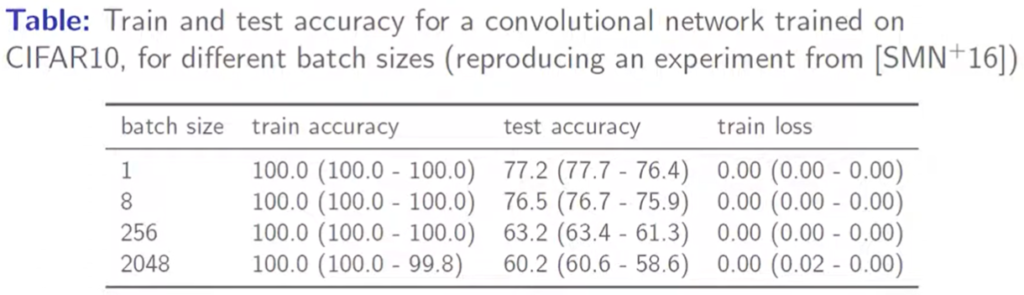 Train and test accuracies on CIFAR10
Based on this observation, it was clear that we need to perform optimization while considering a quantity that correlates well with the generalization. In the past, various norms of weights, as well as sharpness, were considered for this metric, and sharpness was observed to correlate better with the generalization of a model.
The sharpness is a measure of the presence of large changes in loss over small changes in weights.
Sharpness-based generalization bounds
One way to use the properties of sharpness is to define a new loss that’s based on the sharpness. The authors define an expression that is guaranteed to be greater than or equal to the true loss. Let me first introduce this inequality, and I’ll discuss what each term means afterward.
This may look scary at first, but let’s break it down.
First, the left-hand side. $L_\mathscr{D}(w)$ refers to the true loss if the current model was used to calculate the loss against the entire distribution of possible inputs. Of course, we can’t calculate this because we don’t have all the possible data we may encounter. Instead, we use our training set S, a sample from the distribution D.
Now, we come to the right-hand side. Here, we are trying to find the maximum possible loss over a range of epsilon ε. The range is defined to be $||ε||_2 ≤ ρ$, where rho ρ is some constant and the term $||ε||_2$ refers to the L2 norm of ε.
Next, let’s look at the two terms inside the max. The first term refers to the training loss observed when w is displaced by ε. Since we’re taking the max over the values, the first term essentially gives us the maximum training loss in the proximity of our current weights w.
The second term is a weight decay regularization term. Its purpose is to penalize weights being too large. Here, the function h is usually the identity function but it doesn’t have to be, as long as it’s strictly increasing ($x_1 > x_2$ implies $h(x_1) > h(x_2)$).
A more intuitive formulation
The formula discussed in the previous section doesn’t have an explicit term for sharpness. The authors rearrange the formula such that this is more apparent.
Now, we can see that the first term within the formula gives us a clear formulation for sharpness: The maximum difference between the loss from the current weights and the losses near the current weights.
The authors also propose using the standard L2 regularization for the h term ($λ||w||_2^2$). Putting all this together, we arrive at the following objective function (a.k.a. the SAM objective function).
The SAM objective function
This may also look scary but let’s look at it bit by bit. Our objective is to find the weights ($w$) that minimize our loss. This is impacted by two terms: the SAM loss and the regularization term. The regularization term, as previously mentioned, is just to prevent the problem of exploding weights.
As for the SAM loss, we can drop the $L_s(w)$ term since we’re taking the max over varying $ϵ$, and $L_s(w)$ is not dependent on $ϵ$. So, we’re trying to penalize the weights by finding the maximum value of the loss function and then trying to minimize this maximum value.
As you can see, this is a min-max problem: first, we try to maximize a value; then we try to minimize this maximum value. So, how do we solve this?
A closed-form solution
As part of the solution, it is required to first identify the optimal value of $ϵ$ (a.k.a $ϵ^*$). This is defined as follows:
Solving this argmax isn’t too straight forward. The authors approach this problem by linearizing the above solution for $ϵ^*$ using a first-order approximation (a.k.a. the first-order Taylor polynomial).
The result of this approximation is as follows:
I would recommend trying the approximation yourself and seeing if you arrive at the above expression.
Once again, we can simply drop $L_s(w)$ since it does not depend on $\epsilon$. So, we end up with the following.
Turns out this is in the form of something known as the dual norm problem and it has a well-known solution:
If you want to learn how you can move between the problem and solution from the last 2 equations above, take a look at this discussion.
The SAM gradient
Now that we have the optimal value of ϵ, we can calculate the gradient.
Once again, we end up at a somewhat scary-looking equation. In fact, the second term is a bit difficult to compute since it has a 2nd order derivative ($d(ϵ(w))$ is a 2nd order derivative since $ϵ(w)$ also has a derivative of $L_s$ in its definition). While it can be solved using something known as a Jacobian-vector Product (JvP), the computation is slower.
Due to these reasons, the authors tried dropping the 2nd term and it turns out that this does not significantly impact the performance. In certain cases, they observed that dropping the term helps performance as well. Therefore, we finally end up at the following approximation:
Therefore, the gradient of the SAM loss can be approximated to be the gradient of the regular loss evaluated at the perturbed weights ($w+\hat\epsilon(w)$).
Illustration
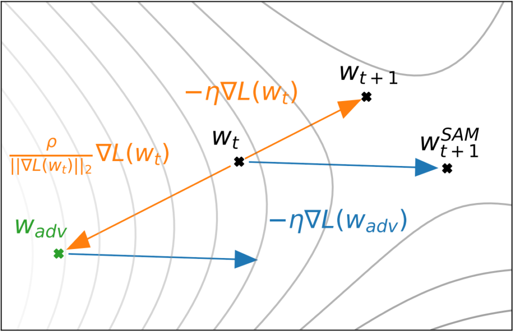 Illustration of SAM
The above diagram from the paper demonstrates how SAM works in contrast to regular gradient descent. The arrow from $w_t$ to $w_{t+1}$ illustrates the step taken through regular gradient descent. In contrast, in SAM, we identify the gradient descent step as taken from wadv (=$w+\hat\epsilon(w)$). However, instead of taking this step from $w_{adv}$, we update $w_t$, the original weights.
Conclusion
That’s about it for the theoretical aspects of SAM. If you would like to learn more about how SAM performs empirically, derivatives of SAM, and open problems, do check out their video on the paper.
If you wish to read more posts on AI math, feel free to check them out here.