Actor-Critic Methods - A Quick Introduction (with Code)
Actor-critic methods are a popular approach to reinforcement learning, which involves the use of two separate components: the actor and the critic. The goal of the actor is to learn a policy that maximizes the expected reward, while the goal of the critic is to learn an accurate value function that can be used to evaluate the actor’s actions.
In this blog post, I’ll mainly explain in the context of TD Actor-Critic. However, the main ideas here can be easily adapted to most other actor-critic methods.
- Temporal Difference (TD) Learning
- The Actor-Critic Algorithm
- Limitations of Actor-Critic Methods
- Implementation of Actor-Critic
- Final Thoughts
Temporal Difference (TD) Learning
Before looking into actor-critic methods, let’s take a look at temporal difference learning.
Note: For all the below examples, I’m using the state-value function (V). Instead, you can also use the action-value function (Q).
Temporal difference (TD) learning is a model-free reinforcement learning algorithm that updates the estimated values of states or state-action pairs based on the difference between the predicted reward and the observed reward. The idea is to learn the values of states or state-action pairs by using the observed reward signal and the estimated values of future states. The equation for TD learning is given by:
where:
-
$V(S_{t})$ is the estimated value of state $S_t$
-
$α$ is the learning rate, a small positive value that determines the size of the update
-
$R_{t + 1}$ is the observed reward at time $t+1$
-
$\gamma$ is the discount factor, a value between 0 and 1 that determines the importance of future rewards
-
$V(S_{t + 1})$ is the estimated value of the next state $S_{t+1}$
The equation is used to update the estimated value of the current state based on the observed reward and the estimated value of the next state. Essentially, with time, V($S_{t}$) should get closer and closer to Rt+1 + $\gamma V(S_{t + 1})$. This means our estimation of the value of the state is getting more and more accurate.
If any part isn’t clear, check out this video for a great introduction to TD learning and model-free reinforcement learning in general. It’s a bit long, but I’d say it’s definitely worth the time.
The Actor-Critic Algorithm
Now that you (hopefully) have a good understanding of TD learning, let’s discuss how it’s used in actor-critic methods.
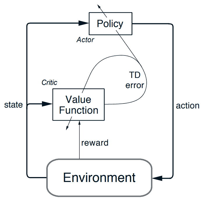 The Actor-Critic Architecture as given in the RL Book by Sutton and Barto
The actor and the critic are typically implemented as neural networks. The actor maps the states to the action probabilities, while the critic maps the states to the state value.
TD Error
The TD error can be defined by the following formula:
You can think of it as the error made by the agent in predicting the value of the current state. Accordingly, the critic update tries to change its network such that this error is lower, while the actor update uses this error as a signal of how much better or worse the chosen action turned out compared to what the critic expected.
Critic Update
Since the critic predicts the value of the state, we can directly use the TD error as the loss. We always want to reduce the TD error, so we square it so that we can minimize it with gradient descent.
Accordingly, the resulting update to the parameters can be given by the following equation:
where,
-
$w$ is the set of parameters of the critic network
-
$\beta$ is the learning rate
-
$\delta$ is the TD error
-
$\nabla_{w}V(S,w)$ is the gradient of the value function (the critic network) with respect to w
You don’t really need to worry about the specifics of the above function since PyTorch handles all the differentiation work. However, if you’re familiar with calculus, try differentiating the square of the TD error while treating the target $R_{t + 1} + \gamma V(S_{t + 1})$ as a constant (as is standard in TD learning), and see if you arrive at the same update (i.e. $\delta \nabla_{w}V(S,w)$, up to a constant factor).
Actor update
To update the actor-network, we can use the probability of the action selected by the network (i.e. $π_θ(a\∣s)$). Now, if the action the actor took was better than what the critic expected, then we would end up with a positive error. So, in this case, we want the loss to be lower. On the other hand, if the action was worse than what the critic expected, then we would end up with a negative error and we want the loss to be higher. One loss function that can satisfy this criterion is the following:
However, in practice, we use the log probability instead because it tends to be more stable and the math works out nicely.
This loss function is one that has been adapted from Policy Gradients. Take a look at this blog post, if you want more background on that.
This results in the following update rule:
where
-
$θ$ is the set of parameters of the actor-network
-
$α$ is the learning rate
-
$δ$ is the TD error
-
$π_θ(a\∣s)$ is the probability of selecting action $a$ from state $s$ as determined by policy $π_θ$
Limitations of Actor-Critic Methods
-
High Variance: The actor-critic algorithm uses the observed reward signal to update the policy and value function. This approach can lead to high variance in the estimates, especially when the reward signal is sparse or noisy.
-
Slow Convergence: The actor-critic algorithm is a model-free reinforcement learning algorithm, which means that it does not use a model of the environment. This makes it slower to converge compared to model-based methods.
-
Function Approximation Error: The actor and critic networks in the actor-critic algorithm are typically implemented as neural networks that approximate the policy and value function, respectively. The approximation error in these networks can affect the quality of the learned policy and value function.
-
Sensitivity to Hyperparameters: The actor-critic algorithm is sensitive to the choice of hyperparameters such as the learning rates for the actor and critic, the discount factor, and the architecture of the neural networks. Choosing the right hyperparameters is important for the success of the algorithm, but it can be difficult in practice.
-
Non-stationarity: The environment in reinforcement learning is non-stationary, meaning that the transition probabilities and rewards can change over time. This can make it difficult for the actor-critic algorithm to learn the optimal policy, especially if the changes are sudden or large.
Implementation of Actor-Critic
Imports
import gymnasium as gym
import numpy as np
import torch
import torch.nn as nn
import torch.optim as optim
-
**gymnasium**- It is the latest version of OpenAI Gym which is a python package for developing and testing learning agents. -
**numpy**- We use NumPy for selecting a random action according to a probability distribution. -
**torch**- We use PyTorch for a number of things like defining our actor-critic network, training it, and calculating the loss.
The Actor-Critic Network
# Define the actor-critic network
class ActorCritic(nn.Module):
    def __init__(self, state_dim, action_dim):
        super(ActorCritic, self).__init__()
        self.fc1 = nn.Linear(state_dim, 64)
        self.fc2 = nn.Linear(64, 64)
        self.fc_pi = nn.Linear(64, action_dim)
        self.fc_v = nn.Linear(64, 1)

    def forward(self, state):
        x = torch.relu(self.fc1(state))
        x = torch.relu(self.fc2(x))
        pi = torch.softmax(self.fc_pi(x), dim=0)
        v = self.fc_v(x)

        return pi, v
Here, we define the actor-critic network. If you look at the forward() method, you’ll notice that there are two outputs. The first output ($\pi$) is the actor output, a.k.a. the action probabilities. Similarly, the second output ($v$) is the critic output, a.k.a. the state value.
I have decided to get both of these outputs from a single network. This is because, in general, this approach tends to be (but not always) more stable than having separate networks for the actor and critic. However, it’s completely fine to try out separate networks, as well.
Essentially, the first two layers create a representation of the state and the two output layers map this representation to our desired outputs. A larger network would be able to hold a better representation but would take longer to train.
Variables for Training
# Define the environment and other parameters
env = gym.make('CartPole-v1')
num_episodes = 1000
discount_factor = 0.99

learning_rate = 0.001

# Initialize the ActorCritic network
agent = ActorCritic(env.observation_space.shape[0], env.action_space.n)

# Define the optimizer
optimizer = optim.Adam(agent.parameters(), lr=learning_rate)
-
**env**- This is the instance of the environment. Here, we’re using the CartPole environment provided by the gym. -
**num_episodes**- This is the number of episodes we’re simulating the environment. Here, I’m initializing it to 1000, but you may need more or less than that. -
**discount_factor**- As mentioned earlier, this is the amount by which we reduce any future rewards. -
**learning_rate**- This is the learning rate for updating the network parameters. This value is being used by the optimizer. -
**agent**- This is our actor-critic network. We give to it, as input, the size of state space and the size of the action space. -
**optimizer**- We use the optimizer to update the network parameters. We give to it, as input, the agent’s parameters and the learning rate.
Training
# Define the training loop
for episode in range(num_episodes):
    # Initialize the environment
    state, _ = env.reset()
    done = False
    total_reward = 0

    while not done:
        # Select an action using the agent's policy
        probs, val = agent(torch.tensor(state, dtype=torch.float32))
        action = np.random.choice(np.arange(len(probs)), p=probs.detach().numpy())

        # Take a step in the environment
        next_state, reward, done, _, _ = env.step(action)
        total_reward += reward

        # Calculate the TD error and loss
        _, next_val = agent(torch.tensor(next_state, dtype=torch.float32))
        err = reward + discount_factor * (next_val.detach() * (1 - done)) - val
        actor_loss = -torch.log(probs[action]) * err.detach()
        critic_loss = torch.square(err)
        loss = actor_loss + critic_loss

        # Update the network
        optimizer.zero_grad()
        loss.backward()
        optimizer.step()

        # Set the state to the next state
        state = next_state

    # Print the total reward for the episode
    print(f'Episode {episode}: Total reward = {total_reward}')
At a high level, we do the following at each episode:
-
We begin by resetting the environment and the other variables.
- Until the episode ends, we:
-
Select an action using the agent’s policy
-
Take a step in the environment using the action
-
Calculate the TD error and thereby, the loss
-
Update the network parameters using the loss
-
Set the new state as the current state
-
- Finally, print the episode number and the total reward for the episode.
Final Thoughts
Actor-Critic is another type of algorithm that has led to a lot of significant improvements in the field of RL. I’ll be discussing some of these derivative algorithms in later blog posts. In the meantime, feel free to check out my explanations for several other RL concepts here.