Model-based vs. Model-free Reinforcement Learning - Clearly Explained
At a high level, all reinforcement learning (RL) approaches can be categorized into 2 main types: Model-based and model-free. One might think that this is referring to whether or not we’re using an ML model. However, this is actually referring to whether we have a model of the environment. We’ll discuss more about this during this blog post.
Note: the content of this blog post is largely based on this great video on the overview of RL methods.
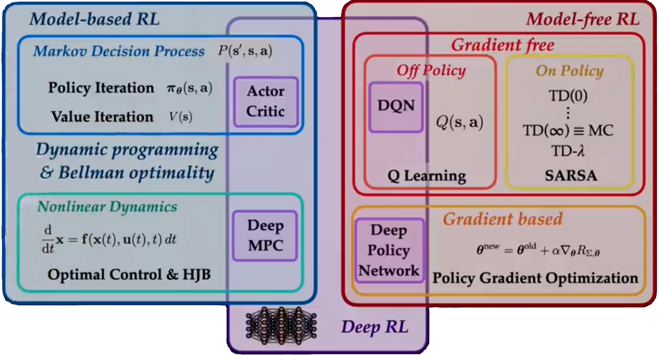 Overview of RL methodologies (source)
- The Reinforcement Learning Problem
- Model-Based Reinforcement Learning
- Model-Free Reinforcement Learning
- Final Thoughts
The Reinforcement Learning Problem
Before we go into details about model-based vs. model-free RL, let me give a bit of background to RL.
Reinforcement learning (RL) is an exciting field of machine learning that deals with training agents to interact with their environments and make decisions to maximize their rewards. It’s like teaching a computer program to learn from its experiences, much like how humans learn from trial and error.
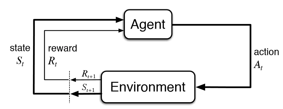 Reinforcement Learning Diagram
There are some key concepts to get us started:
-
Agent and Environment: In RL, we have an “agent” – this is the entity we’re teaching to make decisions. The agent interacts with an “environment” which represents the world or context in which it operates. For instance, the agent could be a robot learning to navigate, and the environment is the physical space it moves in.
-
Actions: The agent can take certain actions, which are the choices it has at any given moment. These actions can be discrete, like moving left or right, or continuous, like the speed at which a robot moves.
-
States: At each step, the agent observes the “state” of the environment. The state is a snapshot that describes the current situation, helping the agent make informed decisions. For example, in a game of chess, the state may include the positions of all the pieces on the board.
-
Rewards: The agent’s goal is to maximize its “rewards”. Rewards are numerical values that represent how well the agent is doing in the environment. Think of them as a score. In a game, a winning move might give a positive reward, while losing might result in a negative one.
-
Policy and Value Function: To make decisions, the agent follows a “policy.” The policy is like a set of rules that dictate which actions to take based on the current state. It helps the agent choose the best actions to maximize its rewards. The “value function” helps the agent evaluate how good a particular state or action is concerning the expected future rewards.
So, in a nutshell, RL is about training an agent to take actions in an environment, learning from the outcomes (rewards), and adjusting its decision-making strategy (policy) to achieve the highest possible rewards.
Model-Based Reinforcement Learning
In this approach, the agent has some knowledge or a “model” of how the environment behaves. Think of this model as a simplified representation of the world that helps the agent make decisions.
Model-based RL may be applied for systems under various conditions such as Markov Decision Processes and Nonlinear Dynamics.
Markov Decision Processes (MDP)
A Markov Decision Process (MDP) is a type of process where the probability of transitioning from one state to another when a specific action is taken is deterministic. Here, the transition probability solely depends on the current state and the chosen action.
In such a case, there are 2 main techniques to optimize the policy: Policy Iteration and Value Iteration. Both these techniques are based on a combination of Dynamic Programming and Bellman’s Equation. I won’t go into too much detail about the 2 methods right now but check out this video if you would like to learn more.
Nonlinear Dynamics
In some cases, the environment is more complex and can’t be described by a simple MDP. Such systems may be representable in terms of differential equations. Instead of using MDP, these situations involve “Nonlinear Dynamics”. The following are two concepts that are commonly referenced in this context.
-
Optimal Control: A control is a variable that an agent uses to manipulate the state. The optimal control is the best sequence of controls that causes some loss function to optimally reduce.
-
Hamilton-Jacobi-Bellman Equation: The Hamilton-Jacobi equation is a mechanics formulation that represents a particle’s motion as that of a wave. Bellman came along and extended this equation to define the Hamilton-Jacobi-Bellman that provides conditions for optimal control, given a loss function. This can be solved to identify the optimal control
Feel free to watch this video if you want a more in-depth understanding of nonlinear dynamics in the context of RL.
While model-based RL has its merits, it does come with limitations. It works well when the agent has a good understanding of the environment, but in many practical situations, building an accurate model is challenging or even impossible. This is where “Model-Free RL” comes into play, as we’ll explore in the next section.
Model-Free Reinforcement Learning
Model-free Reinforcement Learning is an alternative approach when the agent doesn’t have a clear model of the environment. Instead of relying on a predefined understanding of how the world works, the agent learns from its experiences through trial and error. Let’s break down this approach into two categories: Gradient-Free Methods and Gradient-Based Methods.
Gradient-Free Methods
Gradient-free methods are the methods that do not directly optimize the policy estimate using a gradient-based optimization technique.
In Model-Free RL, agents use methods to learn optimal policies directly from interacting with the environment. These methods can be further divided into two main categories: On-Policy and Off-Policy.
On-Policy Algorithms: In On-Policy RL, the agent consistently follows its current policy while exploring the environment. This means it always plays what it thinks is the best game, even if its policy is not yet optimal. On-policy methods include techniques like SARSA, which stands for State-Action-Reward-State-Action. These methods are often more conservative in their learning approach.
Off-Policy Algorithms: Off-policy RL, on the other hand, allows the agent to deviate from its current policy and try different actions. It’s like trying out new strategies even if they seem suboptimal. A key algorithm in this category is Q-learning, which focuses on learning the quality (Q) of taking specific actions in certain states. Off-policy methods can be more efficient and tend to converge faster in learning.
Feel free to take a look at my article comparing Q-learning and SARSA.
Gradient-Based Methods
In Gradient-Based Model-Free RL, agents leverage gradient optimization to directly update the parameters of their policy, value function, or quality function. This approach is often faster and more efficient than gradient-free methods, but it requires knowing the gradients, which may not always be available.
For example, suppose the agent can parameterize its policy using variables (like the weights of a neural network) and understand how these variables affect its expected rewards. In that case, it can use gradient-based optimization techniques like gradient descent to improve its performance. This approach can be highly effective when gradients can be computed, but it may not always be feasible.
Final Thoughts
Model-Based RL relies on having a model of the environment, while Model-Free RL learns directly from experience. Each of these approaches has its strengths and limitations, and the choice of which to use depends on the problem at hand.