Proximal Policy Optimization (PPO) - Explained
Introduced in 2017 by John Schulman et al., Proximal Policy Optimization (PPO) still stands out as a reliable and effective reinforcement learning algorithm. In this blog post, we’ll explore the fundamentals of PPO, its evolution from Trust Region Policy Optimization (TRPO), how it works, and its challenges.
Trust Region Policy Optimization
In one of my previous posts, I discussed an algorithm known as Trust Region Policy Optimization (TRPO). If you have the time, I would recommend that you take a look at the TRPO article. However, for convenience, I’ll give a summary here, as well.
Simply put, TRPO works by preventing updates to the policy network from being too large (take a look at the Policy Gradients article if you’re unfamiliar with policy networks). In other words, for each experience, we’re updating the policy only if the change is a small amount, thereby staying in the “trust region”. This helps with the fact that, usually, when we take an incorrect action, we end up in an irrelevant state and the states observed there onwards are also likely to be irrelevant.
TRPO sidesteps this issue by making sure the probability distribution generated for a given state by the policy doesn’t change too much after each update.
However, turns out TRPO has its limitations. It requires complex and computationally expensive calculations, making it impractical for many real-world applications. PPO managed to simplify the algorithm without sacrificing performance.
PPO Algorithm
The PPO algorithm consists of two high-level processes:
-
Policy Optimization - PPO iteratively collects data by running the current policy in the environment. It then uses this data to improve the policy by maximizing the expected cumulative reward. PPO ensures that the policy updates are within a “trust region” to maintain stability.
-
Value Function Estimation - PPO also estimates the value function to assess the quality of different actions and states. This value function is then used to calculate the Advantage during policy optimization.
When starting out, we initialize the policy and value function using some set of parameters. The goal is to optimize the policy parameters and to help achieve this goal, we also optimize the value function parameters.
PPO Variants
There are two main variants of policy optimization in PPO:
-
PPO-Penalty - TRPO has a hard constraint where if the update is too large, we don’t update the parameters. PPO-Penalty, instead, works by treating the constraint as a penalty (a soft constraint) where the objective function (the thing we want to maximize) is penalized by a large difference in distributions.
-
PPO-Clip - This algorithm works by “clipping” the ratio between the new policy’s distribution and the old policy’s distribution, as defined by the equation below. Through this clipping, we ensure that the ratio between the two policy distributions doesn’t stray too far away from the value 1. We will discuss this algorithm further in the rest of this post as it has been shown to perform better than PPO-Penalty.
 PPO Objective Function
In the above equation, $π_θ$ is the current policy and $π_{θ_k}$ is the old policy. Accordingly, $π_θ(a|s)$ is the probability of taking action $a$ from state $s$ as per the current policy. Furthermore, $A^{π_{θ_k}}$ refers to the Advantage (estimated increase in reward) observed when taking action $a$ from state $s$, estimated under the old policy $π_{θ_k}$. ε is known as the clipping ratio.
So, how exactly does the value of the objective function vary with the value of the ratio? To answer this question, we need to look at two cases.
Case 1: Positive Advantage
A positive advantage implies that the agent’s action was good. So, we want the update to motivate the selection of that action even more. However, we don’t want the update to be too large.
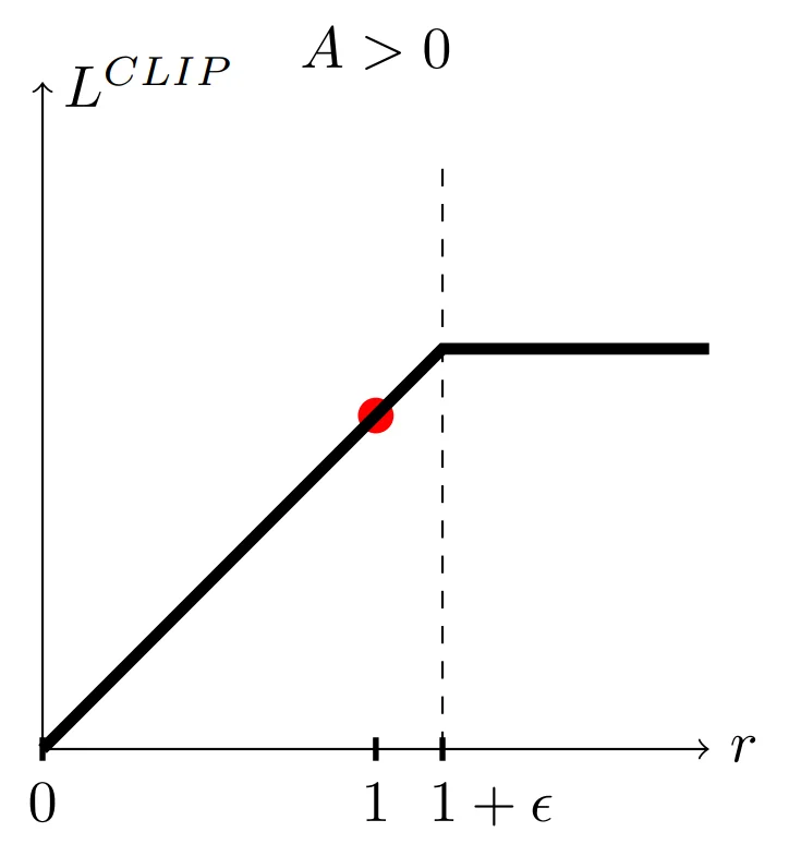 PPO objective function with +ve advantage (source)
In the above graph, the x-axis is the value of the ratio between the two distributions ($r$) and the y-axis is the value of the objective function ($L$).
As long as r remains less than or equal to $1 + ε$, the value of the objective function will be $rA$. Therefore, in this case, the maximum of the objective function is observed when the ratio is $1 + ε$.
We don’t have to be concerned with $1 - ε$ because we’re taking the minimum, so even if $rA$ is less than $(1 - ε)A$, it will not be clipped. This is because we are not worried about the update being too small.
Case 2: Negative Advantage
A negative advantage implies that the agent’s action was bad. So, we want the update to cause the agent to take that action less often for the given state. In other words, we now have a negative value for the objective function and therefore, the updates will be in the opposite direction.
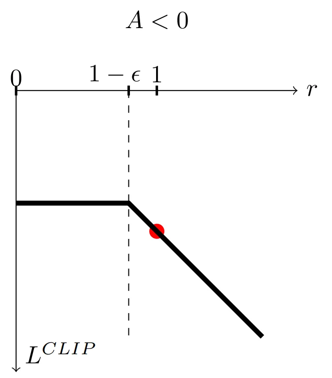 PPO objective function with -ve advantage (source)
As long as r remains greater than or equal to $1 - ε$, the value of the objective function will be $rA$. If r falls below $1 - ε$, the value is clipped at $(1 - ε)A$. Therefore, in this case, the maximum of the objective function is observed when the ratio is $1 - ε$. The further r increases above $1 - ε$, the more negative the value of the objective function. This means the update will try to avoid it, leading to smaller changes in the policy.
Value Function Estimation
Generally, the Value Function gives an estimate of the reward we can expect to gain from the current state (expected return). Training the value function is fairly simple. Since we encounter the actual return at the end of the experience, we can calculate an error. This error can be a function like the mean-squared error.
Summary
The following is the pseudocode for the PPO-Clip algorithm:
-
We begin by initializing the policy and value function parameters.
-
Next, in each iteration, we
-
Collect a set of experiences (states, actions, rewards) using the current policy
-
Use the value function to estimate the advantage
-
Use the objective function to update the policy parameters
-
With regression and gradient descent, update the value function parameters
-
The following image provides a more complete summary:
 PPO-Clip Pseudocode (source)
Challenges of PPO
Hyperparameter Sensitivity
Choosing the right hyperparameters for PPO can be challenging. The algorithm’s performance can vary significantly based on parameter settings like the clipping ratio (ε), making it necessary to perform extensive tuning.
Exploration vs. Exploitation
Balancing exploration (trying new actions to discover better ones) and exploitation (choosing the best-known actions) is a fundamental challenge in RL. PPO tends to become progressively less exploratory as training proceeds, which can lead to getting stuck in local optima.
Final Thoughts
PPO is a powerful RL algorithm, addressing many of the challenges faced by earlier approaches like TRPO. While it has its own set of challenges, PPO’s ability to strike a balance between stability and performance makes it a valuable tool for training agents in various domains.
Hope this helped, and thanks for reading! Feel free to take a look at my other RL-related content here.