Dueling Networks - A Quick Introduction (with Code)
In the past few posts, I discussed the progression of one of the most commonly used Reinforcement Learning algorithms, from Q-Learning to DQNs, to DDQNs. In this post, I’ll give an introduction to another improvement over Deep Q-Networks, known as Dueling Networks. Accordingly, I’ll be covering the following topics:
- Motivation for Using Dueling Networks
- The Architecture of a Dueling DQN
- How Dueling Networks Work
- Advantages of Dueling Networks
- Limitations of Dueling Networks
- Implementation of Dueling Networks
- Conclusion
Motivation for Using Dueling Networks
Traditional Q-learning algorithms can struggle in environments with large state spaces or high-dimensional action spaces. This is because the Q-table must store a value for every possible state-action pair, which can become impractical as the number of states and actions increases.
Deep Q-Networks addressed this issue to a great extent by estimating the state-action mapping using a Neural Network. However, in regular DQNs, the agent chooses the action that is expected to give the best reward. Therefore, only the pathways of the neural network corresponding to the given state and action are updated by backpropagation. As a result, DQNs tend to suffer in cases of large state spaces or action spaces.
However, it turns out that for a given state, the average Q-value of all actions is quite correlated with the Q-value of the best action (see image below). Essentially, this means that the Q-value of the best action is a slight deviation from the average. Thus, regular DQNs have to calculate not only the average, but also the deviation for each action.
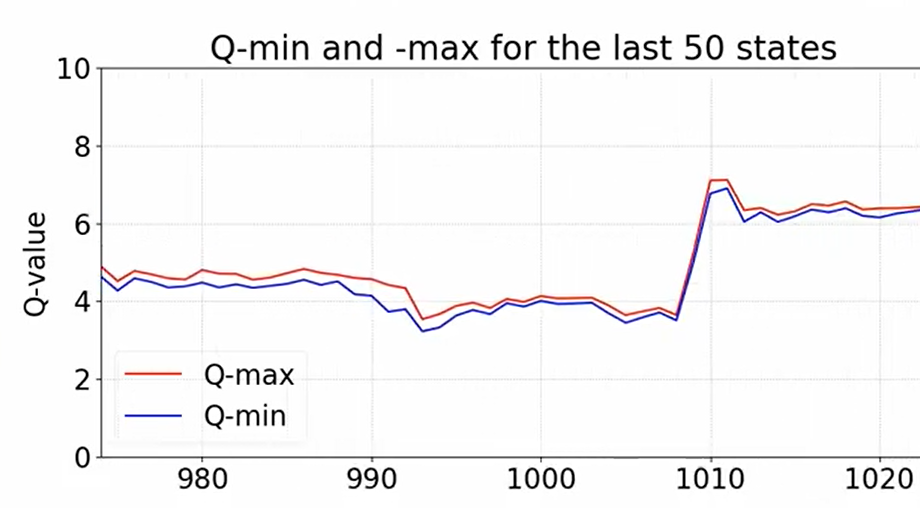 Comparison between Q-min and Q-max (taken from this YT video)
Dueling DQNs address this issue by learning a value function and an advantage function separately. This allows the model to more efficiently capture the relationships between states and actions, as it only needs to learn a single value for each state and a single advantage value for each action, rather than a value for every state-action pair.
In addition to improving the efficiency of the model, learning separate value and advantage functions can also improve the stability of the learning process. This is because the value function provides a baseline prediction for the expected reward of being in a given state, which can help to reduce the impact of noisy or outlier rewards on the learning process.
The Architecture of a Dueling DQN
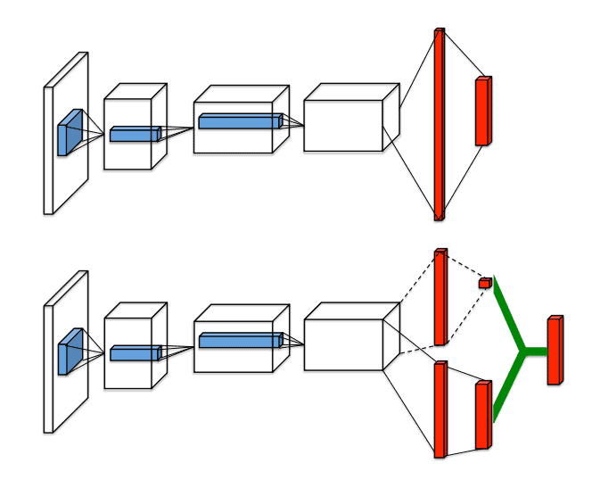 The architecture of DQN (top) vs. Dueling Networks (bottom)
A Dueling DQN consists of two streams that process the input state: a value stream and an advantage stream.
The value stream processes the input state and produces a prediction for the expected future reward of being in that state. This prediction is then passed through a fully-connected layer to produce a single value prediction for the state.
The advantage stream also processes the input state but produces a prediction for the relative value of each action in that state. This is done by passing the processed state through a fully-connected layer that produces a prediction for each action.
The outputs of the value and advantage streams are then combined to produce a prediction for the Q-value of each action in the input state. This is done by subtracting the mean of the advantage predictions from each individual advantage prediction and adding the result to the value prediction.
This can be denoted by:
Q(s,a) = V(s) + [A(s, a) - A(s).mean()]
Or more formally:
 Dueling Network Q-Value formula
The resulting predictions are then used to select the action with the highest Q-value, which is taken by the agent. In addition to the value and advantage streams, a Dueling DQN also includes the usual components of a Q-learning algorithm, such as an experience replay buffer and a target network. We’ll discuss these components and how they fit into the learning process in the next subtopic.
How Dueling Networks Work
A Dueling Network works by learning a value function and an advantage function separately, as described in the previous subtopic. These functions are learned through an iterative process of interacting with the environment and updating the model’s predictions based on the received rewards.
At each time step, the agent receives an input state from the environment and uses the value and advantage streams of the Dueling DQN to predict the Q-values of each possible action.
The action with the highest predicted Q-value is then taken by the agent, and the resulting reward and next state are used to update the model’s predictions. The process of updating the model’s predictions is based on the Bellman equation, which defines the relationship between the expected future reward of a state-action pair and the reward received for taking that action in the current state.
Specifically, the Q-value of a state-action pair is updated to be the sum of the current reward and the discounted future reward of the next state.
To improve the stability and sample efficiency of the learning process, a Dueling DQN also makes use of an experience replay buffer. This is a dataset of past experiences (state, action, reward, next state) that the model can sample from to improve the learning process. By sampling from this dataset, the model can learn from a diverse set of experiences, rather than just the most recent ones.
Advantages of Dueling Networks
Dueling DQNs offer several advantages over traditional Q-learning algorithms. Here are a few key benefits:
-
Improved efficiency: As mentioned previously, Dueling Networks are more efficient than traditional Q-learning algorithms because they only need to learn a single value for each state and a single advantage value for each action, rather than a value for every state-action pair.
-
Improved stability: The separation of the value and advantage streams in a Dueling DQN can also improve the stability of the learning process. The value function provides a baseline prediction for the expected reward of being in a given state, which can help reduce the impact of noisy or outlier rewards on the learning process.
-
Better generalization: Dueling DQNs can also be more effective at generalizing to new situations because they learn a value function and an advantage function separately. This allows the model to better capture the relative value of different actions in a given state, which can be useful for tasks with sparse rewards.
Limitations of Dueling Networks
Like any machine learning algorithm, Dueling Networks have their limitations. Some of the main challenges and limitations of using Dueling DQNs include:
-
Sample efficiency: Dueling DQNs, like other Q-learning algorithms, can require a large number of samples to learn an optimal policy. This can be a challenge in environments where it is difficult or expensive to collect a large number of samples.
-
Stability: While the separation of the value and advantage streams can improve the stability of the learning process, Dueling DQNs can still be sensitive to the choice of hyperparameters and the quality of the training data.
-
Generalization to unseen states: Dueling DQNs can struggle to generalize to unseen states that are significantly different from the states they have encountered during training. This can be a challenge in environments with large state spaces or non-stationary dynamics.
Implementation of Dueling Networks
The implementation below is quite similar to that of DDQN which we discussed in the previous post. We’ve made minor changes in a few places:
-
The QNetwork class has two output layers,
VandA, which represent the value and the advantage, respectively. -
The forward function calculates the output Q-value using both the outputs of
VandA. -
There’s also an
advantagefunction that returns just the advantages of taking each action. -
In the
actmethod of the Agent, we use the aforementioned advantage function for getting the values to pick the best action.
Code
import torch
import torch.nn as nn
import torch.optim as optim
import torch.nn.functional as F
import numpy as np
import random


# Define the network architecture
class QNetwork(nn.Module):
    def __init__(self, state_size, action_size):
        super(QNetwork, self).__init__()
        self.fc1 = nn.Linear(state_size, 64)
        self.fc2 = nn.Linear(64, 64)
        self.V = nn.Linear(64, 1)
        self.A = nn.Linear(64, action_size)

    def forward(self, x):
        x = torch.relu(self.fc1(x))
        x = torch.relu(self.fc2(x))
        x_v = self.V(x)
        x_a = self.A(x)

        return x_v + (x_a - x_a.mean(axis=1, keepdim=True))

    def advantage(self, x):
        x = torch.relu(self.fc1(x))
        x = torch.relu(self.fc2(x))
        return self.A(x)


# Define the replay buffer
class ReplayBuffer:
    def __init__(self, capacity):
        self.capacity = capacity
        self.buffer = []
        self.index = 0

    def push(self, state, action, reward, next_state, done):
        if len(self.buffer) < self.capacity:
            self.buffer.append(None)
        self.buffer[self.index] = (state, action, reward, next_state, done)
        self.index = (self.index + 1) % self.capacity

    def sample(self, batch_size):
        batch = np.random.choice(len(self.buffer), batch_size, replace=False)
        states, actions, rewards, next_states, dones = [], [], [], [], []
        for i in batch:
            state, action, reward, next_state, done = self.buffer[i]
            states.append(state)
            actions.append(action)
            rewards.append(reward)
            next_states.append(next_state)
            dones.append(done)
        return (
            torch.tensor(np.array(states)).float(),
            torch.tensor(np.array(actions)).long(),
            torch.tensor(np.array(rewards)).unsqueeze(1).float(),
            torch.tensor(np.array(next_states)).float(),
            torch.tensor(np.array(dones)).unsqueeze(1).int()
        )

    def __len__(self):
        return len(self.buffer)


# Define the Double DQN agent
class DuelingDQNAgent:
    def __init__(self, state_size, action_size, seed, learning_rate=1e-3, capacity=1000000,
                 discount_factor=0.99, tau=1e-3, update_every=4, batch_size=64):
        self.state_size = state_size
        self.action_size = action_size
        self.seed = seed
        self.learning_rate = learning_rate
        self.discount_factor = discount_factor
        self.tau = tau
        self.update_every = update_every
        self.batch_size = batch_size
        self.steps = 0

        self.qnetwork_local = QNetwork(state_size, action_size)
        self.qnetwork_target = QNetwork(state_size, action_size)
        self.optimizer = optim.Adam(self.qnetwork_local.parameters(), lr=learning_rate)
        self.replay_buffer = ReplayBuffer(capacity)
        self.update_target_network()

    def step(self, state, action, reward, next_state, done):
        # Save experience in replay buffer
        self.replay_buffer.push(state, action, reward, next_state, done)

        # Learn every update_every steps
        self.steps += 1
        if self.steps % self.update_every == 0:
            if len(self.replay_buffer) > self.batch_size:
                experiences = self.replay_buffer.sample(self.batch_size)
                self.learn(experiences)

    def act(self, state, eps=0.0):
        device = torch.device("cuda" if torch.cuda.is_available() else "cpu")
        state = torch.from_numpy(state).float().unsqueeze(0).to(device)
        self.qnetwork_local.eval()
        with torch.no_grad():
            action_values = self.qnetwork_local.advantage(state)
        self.qnetwork_local.train()

        # Epsilon-greedy action selection
        if random.random() > eps:
            return np.argmax(action_values.cpu().data.numpy())
        else:
            return random.choice(np.arange(self.action_size))

    def learn(self, experiences):
        states, actions, rewards, next_states, dones = experiences

        # Get max predicted Q values (for next states) from target model
        Q_targets_next = self.qnetwork_target(next_states).detach().max(1)[0].unsqueeze(1)
        # Compute Q targets for current states
        Q_targets = rewards + self.discount_factor * (Q_targets_next * (1 - dones))

        # Get expected Q values from local model
        Q_expected = self.qnetwork_local(states).gather(1, actions.view(-1, 1))

        # Compute loss
        loss = F.mse_loss(Q_expected, Q_targets)
        # Minimize the loss
        self.optimizer.zero_grad()
        loss.backward()
        self.optimizer.step()

        # Update target network
        self.soft_update(self.qnetwork_local, self.qnetwork_target)

    def update_target_network(self):
        # Update target network parameters with polyak averaging
        for target_param, local_param in zip(self.qnetwork_target.parameters(), self.qnetwork_local.parameters()):
            target_param.data.copy_(self.tau * local_param.data + (1.0 - self.tau) * target_param.data)

    def soft_update(self, local_model, target_model):
        for target_param, local_param in zip(target_model.parameters(), local_model.parameters()):
            target_param.data.copy_(self.tau * local_param.data + (1.0 - self.tau) * target_param.data)
Training the Dueling Network
You can use the code snippet below to train the CartPole task from the OpenAI Gym.
import gym
import numpy as np
from dueling import DuelingDQNAgent
import matplotlib.pyplot as plt

# Create the environment
env = gym.make('CartPole-v0')

# Get the state and action sizes
state_size = env.observation_space.shape[0]
action_size = env.action_space.n

# Set the random seed
seed = 0

# Create the DDQN agent
agent = DuelingDQNAgent(state_size, action_size, seed)

# Set the number of episodes and the maximum number of steps per episode
num_episodes = 1000
max_steps = 1000

# Set the exploration rate
eps = eps_start = 1.0
eps_end = 0.01
eps_decay = 0.995

# Set the rewards and scores lists
rewards = []
scores = []

# Run the training loop
for i_episode in range(num_episodes):
    print(f'Episode: {i_episode}')
    # Initialize the environment and the state
    state = env.reset()[0]
    score = 0
    # eps = eps_end + (eps_start - eps_end) * np.exp(-i_episode / eps_decay)
    # Update the exploration rate
    eps = max(eps_end, eps_decay * eps)

    # Run the episode
    for t in range(max_steps):
        # Select an action and take a step in the environment
        action = agent.act(state, eps)
        next_state, reward, done, _, _ = env.step(action)
        # Store the experience in the replay buffer and learn from it
        agent.step(state, action, reward, next_state, done)
        # Update the state and the score
        state = next_state
        score += reward
        # Break the loop if the episode is done
        if done:
            break

    print(f"\tScore: {score}, Epsilon: {eps}")
    # Save the rewards and scores
    rewards.append(score)
    scores.append(np.mean(rewards[-100:]))

# Close the environment
env.close()

plt.ylabel("Score")
plt.xlabel("Episode")
plt.plot(range(len(rewards)), rewards)
plt.plot(range(len(rewards)), scores)
plt.legend(['Reward', "Score"])
plt.show()
Conclusion
Alright, that’s about it for the Dueling Networks. Let me know if there are any questions. Also, feel free to check out my other RL-related posts here, if you’d like. :-)