Q-Learning and SARSA in RL - Similarities and Differences Explained
Q-learning and SARSA are two of the algorithms that one generally encounters early in the journey of learning reinforcement learning. However, despite the high similarity between these two algorithms, in practice, Q-learning often takes prominence in terms of performance. In this blog post, we’ll discuss the similarities and differences between these two algorithms, as well as the reason for the strength of one over the other.
- Temporal Difference (TD) Learning
- TD(n)
- SARSA
- Q-Learning
- Pros and Cons of Q-Learning and SARSA
- Final Thoughts
Temporal Difference (TD) Learning
Let’s begin by talking about an equation for the value function. We can denote the value of a state as the sum of the reward we get from that state and the value of the next state. Generally, we multiply the value of the next state by a number less than one. We refer to this value as gamma (γ). All this can be denoted by the following equation:
Here, the $\mathbb{E}$ symbol is used to show that we don’t yet know whether we will receive the reward rk or whether our value function is correct.
Turns out, we can use this equation to write a new equation that will act as our update function. In other words, this new equation will tell us what we need to do in order to improve our value function’s estimates.
 Value function update equation
This is also known as TD(0) learning and it’s what Q-learning and SARSA are based on.
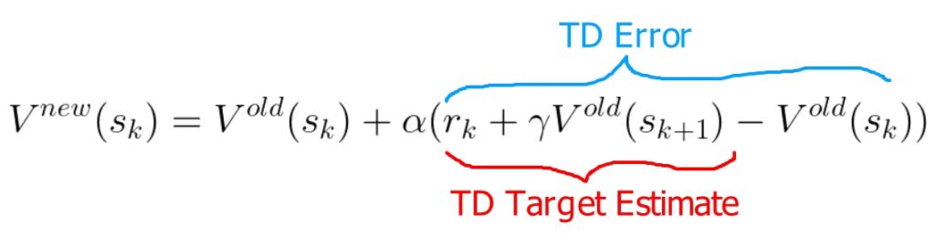
It’s a big-looking equation, so let me break down what’s going on here. On the left, we have the updated value function: the function we get after updating our old value function. On the right, we do the update.
You may also notice a familiar set of terms. $r_k + \gamma V_{old}(s_{k+1})$ is the estimate of the value function that we saw in the previous equation (a.k.a. the target estimate). Here, $r_k$ is the reward we actually received when we went to sk by following some policy. So, the target estimate is likely to be closer to the actual value function than $V_{old}(s_k)$.
But, we don’t want to immediately use that as our new value function. Why?
It’s because it’s still an estimate. We don’t want to accept the result from one experience as the hard truth. Instead, we want to incrementally go towards the correct value function using multiple experiences.
So, what TD-learning does is, it takes the difference between the target estimate and the old value estimate, and uses this difference to update the old value function by some amount. This difference is also known as the TD error. The amount by which we update the function is controlled by $α$.
Let’s look at a simple example. Say the agent did something and it got a better reward than the value function expected. Then, the target estimate is higher than the old estimate. So the TD error would be positive and the update would give a higher value to that state.
TD(n)
This section is not too important to understand Q-learning or SARSA, but it doesn’t hurt to understand what it is. However, feel free to skip it if you wish.
At the beginning of the previous section, you saw an equation for the value function. It was like looking one time-step into the future. Turns out there is actually a recursive nature to this equation that we can use to look more timesteps into the future.
Just as we wrote $V_{old}(s_k)$ as $\mathbb{E}(r_k + \gamma V_{old}(s_{k+1}))$, we can replace $V_{old}(s_{k+1})$ with $r_{k+1} + \gamma V_{old}(s_{k+2})$. Note that we don’t have to include the expectation sign ($\mathbb{E}$) in this substitution because the outer $\mathbb{E}$ already captures the idea. So, now we get the following equation.
Substituting this back into our update equation gives us the following.
As you might have guessed, we can do this expansion as many times as we want. This would give us the following target estimate.
where n is the number of expansions since the first value function estimate.
Substituting it into the update equation, we get the update equation for TD(n).
Substituting back $n=0$, we get our initial update equation from the previous section.
SARSA
Now that you have an idea of what TD learning is, we can easily transition to what SARSA is. SARSA is the on-policy TD(0) learning of the quality function (Q).
The quality function tells you how good some action is when taken from a given state. All the equations we previously discussed for value functions (V) are also applicable to quality functions (Q). The only difference is that now we’re taking 2 inputs (state s and action a) instead of just the state s.
Notice how this equation is essentially the same as the TD(0) equation, with the exception that now we’re working with the quality function rather than the value function.
In the SARSA algorithm, we’re working with the current State ($s_k$), Action taken from the current state ($a_k$), Reward observed after taking the action ($r_k$), the next State after taking the action ($s_{k+1}$), and the Action to take from the next state ($a_{k+1}$).
So, why do we call it on-policy? This is because the policy that resulted in the action ak is the same policy that we’re using to find $a_{k+1}$.
An algorithm is known as off-policy when the behavior policy and the target policy are different, and on-policy when they are the same. The behavior policy is the policy used to perform the actions and generate experiences, while the target policy is the policy that is being optimized by the algorithm, based on the experiences from the behavior policy.
Q-Learning
Q-learning is the off-policy TD(0) learning of the quality function (Q).
Let’s take a look at the Q-learning update equation. First, compare it against the SARSA update equation and identify what the difference between them is.
Look at the TD target estimate. Instead of $r_k+ \gamma Q^{old}(s_{k+1}, a_{k+1})$, we are now taking the maximum Q-value over all the actions we can take from state $s_{k+1}$.
So, what makes the Q-learning algorithm off-policy? Turns out, in Q-learning, the behavior policy (the policy that generated the reward $r_k$) need not be the same as the target policy (the policy that chooses the action that gives the maximum Q-value). The target policy can try to choose the optimal action (exploitation) without sacrificing exploration because the behavior policy could still act suboptimally with better exploration.
If you still have doubts about how Q-learning works, take a look at this blog post for a more thorough explanation.
Pros and Cons of Q-Learning and SARSA
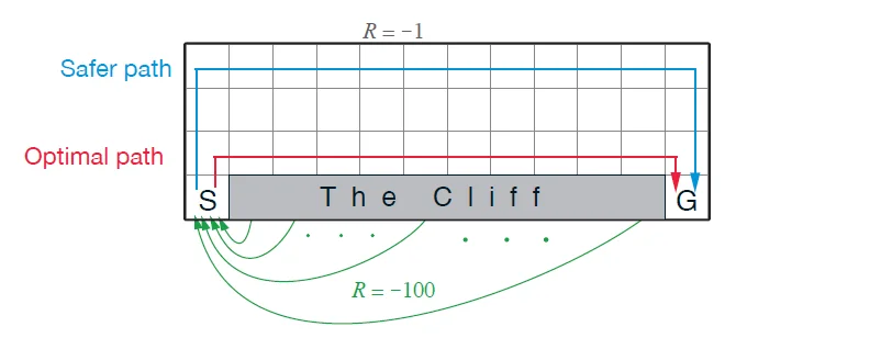 Comparison of the safe path (SARSA) vs. optimal path (Q-learning) (source)
-
Global Optimum: Given sufficient exploration, Q-Learning will reach the globally optimal policy. SARSA, on the other hand, will require the exploration to be reduced with time in order to reach the optimal policy. For instance, the epsilon value in epsilon-greedy SARSA would have to be reduced with time. It can be a hassle to tune this hyperparameter.
-
Conservative Path: On the other side of the spectrum, SARSA tends to identify the safer path compared to Q-learning. Take a look at the above image (cliff walking). This conservativeness happens because the exploration steps (random actions) near the cliff also contribute to updating the policy and as a result, the algorithm believes that there is a risk in staying near the cliff.
-
Convergence: In Q-learning (and in off-policy algorithms in general), there samples tend to have a higher variance. This is because the action proposed by the behavior policy may be different from that of the target policy. As a result, Q-learning is likely to take longer to converge.
Final Thoughts
Hope this helps. If you would like to see more explanations for reinforcement learning concepts, check out the RL page of the blog.