Trust Region Policy Optimization (TRPO) - A Quick Introduction
Trust Region Policy Optimization (TRPO) is a Policy Gradient method that addresses many of the issues of Vanilla Policy Gradients (VPG). Despite not being state-of-the-art currently, it paved the path for more robust algorithms like Proximal Policy Optimization (PPO).
Completely understanding TRPO requires a bit of math which I won’t bore you too much with. Instead, I’ll link to any resources (for the math concepts) that you can refer to learn those concepts.
In this blog post, I hope to cover the following:
Why TRPO?
Imagine that you’re on the mountain slope below. I know it’s a weird-looking mountain but bear with me.
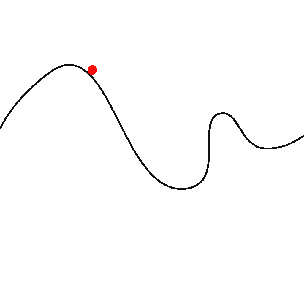 Gradient Descent mountain
Gradient descent will tell us that we need to take a step to the right, in this case. If we take a regular step to the right, it’s alright. We’re still taking a step toward the optimal policy. However, if we take a slightly larger step, we end up in an entirely different pit. We generally don’t want that.
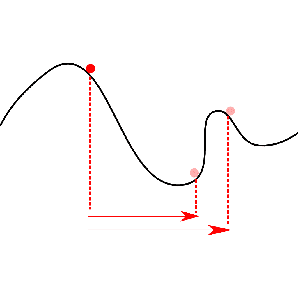 Gradient Descent mountain - large and small steps
In supervised learning, this is usually not too big of a problem because we have the correct label for all our data. So, even if we step out of our initial pit because of one label, we are usually brought back in by the remaining labels.
However, this is usually not the case with reinforcement learning. If we take a wrong step in gradient descent, our outputs may lead to an incorrect action. This incorrect action may then take us to a bad state. All experiences from here on out, until the end of the episode, may well be pointless.
It’s more difficult to recover from this because the data we get for training depends on the current policy. Since the policy is constantly changing, we can say that the data is non-stationary. In other words, the data being trained after each epoch is different.
This is where TRPO comes in. The first two words of the phrase “Trust Region Policy Optimization” gives an intuition of what it does. Simply put, the main idea is to limit the difference between our current policy and the new policy. “Trust Region” refers to this space around the predictions of our current policy which we “trust” to be an acceptable prediction.
How TRPO works
Let’s also take a quick look at the objective function that TRPO uses (a.k.a. the surrogate advantage).
Objective function
 Surrogate Advantage (source)
The above objective function attempts to estimate the advantage of the updated policy based on the advantage observed in the old policy. This concept is known as importance sampling. Put simply, we’re making the assumption that the ratios between the two probability distributions are equal to the ratios between the two advantages.
Anyway, we want to maximize this objective function (because we want to maximize the advantage of the action we take). But, we also don’t want to stray too far from our current policy.
KL Divergence
So how does TRPO do that? This is done by using something called the Kullback-Leibler (KL) divergence between the predicted distributions of the old policy and the new policy for a given state.
Note: Oversimplifying a bit, the KL divergence is a way to measure how different one probability distribution is compared to another. Take a look at this stack exchange question to get a good intuition.
 KL Divergence formula
In the case that P(x) and Q(x) are equal, the log of the ratio of the two probabilities would be equal to log(1) or 0. The larger the difference between the distributions for a given action, the larger the divergence is. By multiplying each log ratio by P(x), we are essentially weighting the divergence for a given action with the probability of picking that action.
You don’t have to worry too much about the equation. I’m just mentioning it to give familiarity in case it comes up elsewhere.
Optimizing
Let’s look at how all this comes together.
We want to maximize the surrogate advantage. But, when maximizing it, the new policy can deviate a lot from the old policy. This can lead to the problems which we talked about in the beginning.
To avoid this, we look at the KL divergence. We only update our parameters if the KL divergence is below a certain value.
All this can be summarized into the following equation.
 TRPO update equation (source)
where,

In other words,
-
We’re trying to maximize the previously mentioned objective function
-
While maximizing, we’re making sure the average of the KL-divergences over the states observed by the old policy remains less than some value.
Natural Policy Gradients (NPG) vs TRPO
It turns out that everything I discussed so far applies to both NPG and TRPO. However, there are differences between NPG and TRPO when it comes to the implementation/practical side of things. In fact, TRPO is an improvement over NPG.
Below I will discuss further the factors that separate the two algorithms. However, if you came for the high-level concepts behind TRPO and don’t care much for its practical details, then feel free to skip this section.
NPG
In practice, it is difficult to directly use the equations we previously mentioned. Instead, we use Taylor approximations of the objective function and the constraint. This results in the following:
 Taylor approximated objective function and constraint (source)
where g is the 1st order derivative of the objective function and H is something known as the Hessian Matrix or the Fisher Information Matrix of the distribution KL-divergence among the states. This is still an intermediate step, so you don’t have to worry too much about the definitions if you don’t want to.
Note: The Hessian matrix is an N-by-N matrix, where N is the size of the parameter vector θ. This matrix gives the derivative of a function with respect to any two parameters of the function.
Now, we can use this objective function and the constraint to define the parameter update using something known as Lagrangian Duality.
Note: Lagrangian Duality is a concept used to solve problems of the above nature where we have a function we want to optimize and we have one or more constraints we want to satisfy. This video gives a pretty good introduction to this concept.
Update Rule
This results in the following update rule:
 NPG Update Rule (source)
This is the idea behind Natural Policy Gradients. However, there are several drawbacks to this.
-
The usage of Taylor approximation leads to an error, especially since it assumes that θold is very close to θ. As a result, θ may violate the constraint given by the KL-divergence.
-
Since the Hessian Matrix is of size N-by-N, a large parameter vector would lead to an exponentially large matrix. As you can imagine, this would not only consume a lot of memory, but when it comes to getting H-1, it would take a huge amount of time (O(N3) to be exact).
This is where TRPO comes in.
TRPO
TRPO solves each of the two previously mentioned problems as follows:
Preventing constraint violation
To make sure θ doesn’t violate the constraint, we introduce another term known as alpha (α), where α is between 0 and 1.
 TRPO Update Rule (source)
where j is the smallest integer that keeps the result within the constraint. The larger j is, the smaller αj is, the less the new θ deviates from the old θ. So, we basically start with j = 1, and then increment j one by one until we arrive at a value where the constraints are satisfied. This process is also known as backtracking line search.
Dealing with the size of the Hessian Matrix
If you look at the update rule, you may notice that the Hessian matrix always occurs with another term (H-1g). Therefore, what we need to find is x=H-1g. This can be rewritten as Hx=g by multiplying both sides by H.
Turns out, you can directly solve for x without calculating the whole Hessian matrix. To do this, we use something known as the conjugate gradient method.
Note: The conjugate gradient method is an algorithm to iteratively solve a linear system of equations. By using an iterative approach, we avoid having to calculate the entire Hessian matrix as opposed to the direct approach. In our case, the algorithm solves the equation Hx=g. Take a look at this video for a step-by-step explanation of how the algorithm works.
Complete Algorithm
The complete algorithm can be denoted by the following pseudocode:
 TRPO Complete Pseudocode (source)
Final Thoughts
As I mentioned at the beginning of the post, despite the effectiveness that TRPO brought with it, PPO has succeeded in improving it further to the point of being state-of-the-art. However, it is good to have an idea of how the algorithm reached its current state.
Hope this helped, and thanks for reading! Feel free to take a look at my other RL-related content here.