Policy Gradient - A Quick Introduction (with Code)
Policy Gradient is one of the most fundamental algorithms in Reinforcement Learning that has led to a number of state-of-the-art algorithms. It was first introduced by Richard Sutton et al. in the paper “Policy Gradient Methods for Reinforcement Learning with Function Approximation”. In this blog post, I’ll discuss the basic principles behind Policy Gradient. Accordingly, I’ll be covering the following subtopics:
- What is a Policy?
- The Policy Network
- Policy Gradient in Simple Terms
- Policy Gradient Implementation with PyTorch
- Conclusion
What is a Policy?
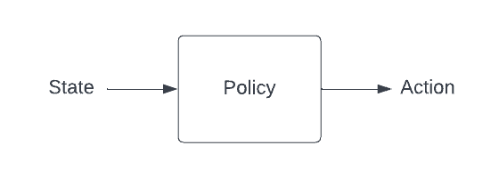
Policy Diagram
In reinforcement learning, the policy is a function that maps a given state to an action.
One way to think of the problem of reinforcement learning is to say that it’s the task of identifying the best possible policy. Policy gradients is a technique to do this identification.
The Policy Network
In the previous posts, I discussed Q-networks, where a neural network is used to predict the value of taking a certain action (action-values/q-values). A policy network on the other hand directly plays the role of a policy. In other words, given a certain state, it outputs the probability of taking each action. This can either be a discrete set of actions of a continuous distribution.
Note: Generally, the output of the policy network is considered to be the log probability rather than the regular probability. This is because using the log probability tends to converge better when training.
Policy Gradient in Simple Terms
Let’s begin by taking a look at supervised learning. Supervised learning is a type of machine learning where you have the actual labels for your dataset.
We can formulate a given reinforcement learning task as a supervised learning task by assuming that we know beforehand, which actions were the best for each state in the training state. However, in reality, this assumption is often wrong.
On the other hand, we do have the option to know how good the actions we took were. This feedback can be inferred from the rewards we receive during training.
Accordingly, in order to improve our policy network, we need to maximize the probability of choosing actions that worked and minimize the probability of choosing actions that didn’t work.
To do this, we scale the predicted (log) probabilities by the reward and try to maximize this result (or rather, minimize the negative of this result). This is how Vanilla Policy Gradients (a.k.a. VPG or REINFORCE) works.
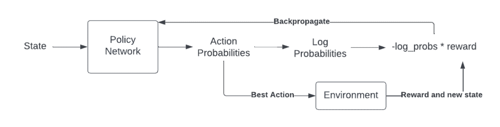
Policy Gradient Diagram
If you’re interested in the exact derivation of this gradient, take a look at the following proof.

Derivation of the objective function for Basic Policy Gradient (source)
Policy Gradient Implementation with PyTorch
Imports
import gym
import torch
import torch.nn as nn
import torch.optim as optim
The Environment

Cart Pole task from OpenAI gym
The code starts by importing the necessary libraries and creating the environment. In this case, the environment is the CartPole-v1 environment from the OpenAI Gym library. This environment consists of a pole that is attached to a cart. The agent’s goal is to balance the pole by moving the cart left or right.
env = gym.make("CartPole-v1")
The Policy Network
The policy function maps states of the environment to actions. In this implementation, the policy function is a neural network with two linear layers and a softmax output layer. The first layer has 32 hidden units and the second layer has 2 output units. The first layer takes in the state of the environment, and the second layer outputs the probability of taking each action.
# Get the state and action sizes
state_size = env.observation_space.shape[0]
action_size = env.action_space.n

# Define the policy network
class Policy(nn.Module):
    def __init__(self):
        super(Policy, self).__init__()
        self.fc1 = nn.Linear(state_size, 32)
        self.fc2 = nn.Linear(32, action_size)

    def forward(self, x):
        x = torch.relu(self.fc1(x))
        x = self.fc2(x)
        return torch.softmax(x, dim=-1)

policy = Policy()
The Loss Function and Optimizer
loss_fn = nn.CrossEntropyLoss()
optimizer = optim.Adam(policy.parameters())
The loss function and optimizer are defined next. The loss function is the cross-entropy loss and the optimizer is the Adam optimizer. The optimizer is used to update the parameters of the policy function.
The Update Policy Function
def update_policy(rewards, log_probs, optimizer):
    log_probs = torch.stack(log_probs)
    loss = -torch.mean(log_probs * (sum(rewards) - 15))
    optimizer.zero_grad()
    loss.backward()
    optimizer.step()
The update_policy function takes in the rewards, the log probabilities of the actions taken in the episode, and the optimizer for updating the policy’s parameters.
First, we stack the log_probs because it’s currently a list of tensors, whereas what we need is a single tensor (for getting the mean).
Before getting the mean, I’ve used a very simple technique to weigh the `log_probs`. I’ve used the sum of rewards during the episode to indicate how much the actions of the episode helped. I went for this simple approach because the reward is always one for each step of the Cartpole task, by default. Please update this line as per the problem.
Finally, we use the optimizer to update the parameters of the policy function using the calculated loss.
Training Loop
The training loop starts by resetting the environment, then the agent takes random actions and the rewards and log-probabilities of the actions are collected during the episode. When the episode ends, the policy is updated using the rewards and log-probabilities of the actions. The training loop repeats this process for a fixed number of episodes.
# Training loop
for episode in range(10000):
    state, _ = env.reset()
    done = False
    rewards = []
    log_probs = []

    while not done:
        # Select action
        state = torch.tensor(state, dtype=torch.float32).reshape(1, -1)
        probs = policy(state)
        action = torch.multinomial(probs, 1).item()
        log_prob = torch.log(probs[0, action])

        # Take step
        next_state, reward, done, _, _ = env.step(action)
        rewards.append(reward)
        log_probs.append(log_prob)
        state = next_state

    # Update policy
    print(f"Episode {episode}: {sum(rewards)}")
    update_policy(rewards, log_probs, optimizer)
    rewards = []
    log_probs = []
The Combined Code
import gym
import numpy as np
import torch
import torch.nn as nn
import torch.optim as optim

# Create the environment
env = gym.make("CartPole-v1")

# Get the state and action sizes
state_size = env.observation_space.shape[0]
action_size = env.action_space.n

# Define the policy function (neural network)
class Policy(nn.Module):
    def __init__(self):
        super(Policy, self).__init__()
        self.fc1 = nn.Linear(state_size, 32)
        self.fc2 = nn.Linear(32, action_size)

    def forward(self, x):
        x = torch.relu(self.fc1(x))
        x = self.fc2(x)
        return torch.softmax(x, dim=-1)

policy = Policy()

# Define the loss function and optimizer
loss_fn = nn.CrossEntropyLoss()
optimizer = optim.Adam(policy.parameters(), lr=0.01)

# Define the update policy function
def update_policy(rewards, log_probs, optimizer):
    log_probs = torch.stack(log_probs)
    loss = -torch.mean(log_probs) * (sum(rewards) - 15)
    optimizer.zero_grad()
    loss.backward()
    optimizer.step()

gamma = 0.99

# Training loop
for episode in range(5000):
    state, _ = env.reset()
    done = False
    score = 0
    log_probs = []
    rewards = []

    while not done:
        # Select action
        state = torch.tensor(state, dtype=torch.float32).reshape(1, -1)
        probs = policy(state)
        action = torch.multinomial(probs, 1).item()
        log_prob = torch.log(probs[:, action])

        # Take step
        next_state, reward, done, _, _ = env.step(action)
        score += reward

        rewards.append(reward)
        log_probs.append(log_prob)
        state = next_state

    # Update policy
    print(f"Episode {episode}: {score}")
    update_policy(rewards, log_probs, optimizer)
Conclusion
Hope this explanation and code were helpful for anyone getting started with policy gradients. Of course, there have been a lot of improvements to policy gradients over the years. However, it remains to be the starting point of a lot of state-of-the-art techniques.
Feel free to ask any questions in the comments below and check out my explanations for several other reinforcement learning concepts here.