Deep Q-Networks (DQN) - A Quick Introduction (with Code)
In my last blog post, I gave an introduction to Q-learning. One major issue with Q-learning was that it doesn’t work too well when the number of actions or number of states is too large. This is because you would have to maintain a table containing the expected reward (i.e., the sum of future rewards) for every state-action combination, which can take up a lot of space. To address this, researchers proposed the usage of Deep Neural Networks to approximate the expected reward for any state-action combination (action-value). This is what’s known as a Deep Q-Network (DQN).
 Atari Breakout
- Deep Q-Networks and How they work
- Experience Replay
- Advantages and Limitations
- Improvements to DQNs
- Implementing a DQN
- Conclusion
Deep Q-Networks and How they work
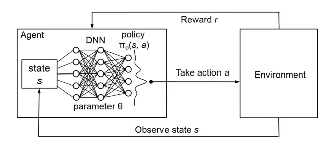 DQN Architecture
Deep Q-Networks (DQNs) are a type of neural network that is used to learn the optimal action-selection policy in a reinforcement learning setting. They were first introduced by Google DeepMind in a 2015 paper called “Human-level control through deep reinforcement learning”. You can get a quick overview of what they did in this video by Two Minute Papers.
DQNs work by using a neural network to approximate the action-value function, which maps states of the environment to the expected return (i.e., the sum of future rewards) for each possible action. The goal of the DQN is to learn the optimal policy, which is the action that will maximize the expected return for each state.
To train the DQN, the agent interacts with the environment by taking actions and receiving rewards and observations. The agent stores these experiences in a memory buffer and periodically updates the DQN using these experiences. The update is done through a process called experience replay, where a batch of experiences is randomly sampled from the memory buffer and used to update the DQN. This process helps the agent to learn from a wider variety of experiences and can stabilize the learning process.
The DQN uses a variant of the Q-learning algorithm, which is an off-policy algorithm that updates the action-value function based on the difference between the predicted value and the target value. The target value is calculated using the Bellman equation, which states that the expected return for a given action is the immediate reward plus the maximum expected return for the next state.
Experience Replay
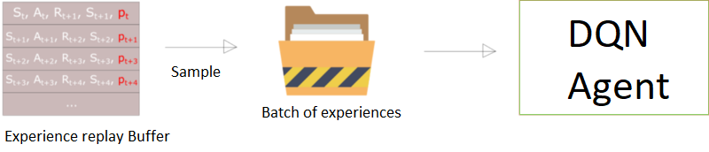 Experience Replay Workflow
Experience replay is a key component of DQNs and other reinforcement learning algorithms that use neural networks. It involves storing a set of experiences (i.e., state-action-reward-next state tuples) in a memory buffer and using these experiences to update the DQN during training.
The main idea behind experience replay is that it allows the agent to learn from a wider variety of experiences, rather than just the most recent ones. This can help to stabilize the learning process and can improve the overall performance of the DQN.
How it works
Experience replay works by randomly sampling a batch of experiences from the memory buffer and using these experiences to update the DQN. This process is done in addition to the normal online updates, where the DQN is updated based on the current state and action. By sampling from a large pool of experiences, the agent is able to learn from a more diverse set of situations, which can improve its overall performance.
Why use it?
One of the main benefits of experience replay is that it helps to decorrelate the experiences in the training data. This is important because the Q-learning algorithm relies on the assumption that the experiences are independent and identically distributed (i.i.d.). By decorrelating the experiences, experience replay helps to satisfy this assumption, which can improve the learning process.
Advantages and Limitations
Advantages
-
DQNs can learn directly from raw sensory input, such as images or audio. This is particularly useful for tasks where the state space is large or continuous, as it can be challenging to manually specify a set of features to describe the state.
-
They can learn directly from the reward signal, without the need for manual reward shaping or expert demonstrations. This can make it easier to specify the reinforcement learning problem and can allow the agent to learn more complex behaviors.
-
DQNs are also relatively sample efficient, meaning that they can learn effectively with relatively few interactions with the environment. This is particularly useful for tasks where the cost of taking an action is high or where it is difficult to gather a large amount of data.
Limitations
-
DQNs can struggle to learn in environments with sparse rewards, where the majority of actions do not result in a reward. This can make it difficult for the agent to learn a good policy, as it may not receive enough feedback to learn effectively.
-
They can be sensitive to the choice of hyperparameters, such as the learning rate and the size of the network. Tuning these hyperparameters can be challenging, and it is important to carefully choose them in order to achieve good performance.
-
DQNs can be computationally intensive, particularly for tasks with high-dimensional state spaces or large networks. This can make it difficult to apply DQNs to certain tasks or may require specialized hardware to achieve good performance.
Improvements to DQNs
There have been several improvements to DQNs over the years, which have helped to address some of the limitations of the original algorithm and have led to better performance on a wider range of tasks. Some of the most significant improvements include:
Double DQN
The original DQN algorithm can suffer from an overestimation of the action-values, which can lead to suboptimal behavior. The Double DQN algorithm addresses this problem by using two separate networks: a target network and a primary network. The primary network is used to select actions, while the target network is used to calculate the target values for the primary network. By decoupling the action selection and value estimation processes, the Double DQN can reduce the overestimation of action-values and improve the learning process.
Dueling DQN
The Dueling DQN architecture separates the value function and the advantage function into separate streams, which can be more efficient for learning in some environments. The value function estimates the expected return for each state, while the advantage function estimates the relative advantage of each action for each state. By learning these two functions separately, the Dueling DQN can more efficiently learn the optimal policy.
Prioritized Experience Replay
In the original DQN algorithm, experiences are uniformly sampled from the memory buffer for training. However, some experiences may be more important than others for learning the optimal policy. Prioritized Experience Replay addresses this problem by prioritizing the sampling of experiences based on their temporal difference (TD) error, which measures the difference between the predicted and target values. This can lead to more efficient learning, as the agent is able to learn more from important experiences.
QR-DQN
QR-DQN is an improvement to DQNs that uses a quantile regression approach to estimate the action-value function. In contrast to the traditional DQN approach, which estimates a single value for each action, QR-DQN estimates a distribution of values for each action. This can help to reduce the overestimation of action-values and improve the learning process.
Rainbow DQN
Rainbow is a combination of several improvements to the DQN algorithm, including the use of Double DQN, Dueling DQN, Prioritized Experience Replay, and several other enhancements. Rainbow has been shown to achieve state-of-the-art performance on a wide range of Atari games and has set several new benchmarks for reinforcement learning.
Implementing a DQN
The implementation of DQN is quite similar to that of regular Q-learning. The main difference is that we now use a neural network instead of the Q-table. Additionally, we also use experience replay, to further improve the performance of our agent.
 Cart Pole task from the OpenAI Gym
The following code implements DQN for the Cartpole task from the OpenAI gym.
import torch
import torch.nn as nn
import torch.optim as optim
import torch.nn.functional as F
import numpy as np
import random


# Define the network architecture
class QNetwork(nn.Module):
    def __init__(self, state_size, action_size):
        super(QNetwork, self).__init__()
        self.fc1 = nn.Linear(state_size, 64)
        self.fc2 = nn.Linear(64, 64)
        self.fc3 = nn.Linear(64, action_size)

    def forward(self, x):
        x = torch.relu(self.fc1(x))
        x = torch.relu(self.fc2(x))
        x = self.fc3(x)
        return x


# Define the replay buffer
class ReplayBuffer:
    def __init__(self, capacity):
        self.capacity = capacity
        self.buffer = []
        self.index = 0

    def push(self, state, action, reward, next_state, done):
        if len(self.buffer) < self.capacity:
            self.buffer.append(None)
        self.buffer[self.index] = (state, action, reward, next_state, done)
        self.index = (self.index + 1) % self.capacity

    def sample(self, batch_size):
        batch = np.random.choice(len(self.buffer), batch_size, replace=False)
        states, actions, rewards, next_states, dones = [], [], [], [], []
        for i in batch:
            state, action, reward, next_state, done = self.buffer[i]
            states.append(state)
            actions.append(action)
            rewards.append(reward)
            next_states.append(next_state)
            dones.append(done)
        return (
            torch.tensor(np.array(states)).float(),
            torch.tensor(np.array(actions)).long(),
            torch.tensor(np.array(rewards)).unsqueeze(1).float(),
            torch.tensor(np.array(next_states)).float(),
            torch.tensor(np.array(dones)).unsqueeze(1).int()
        )

    def __len__(self):
        return len(self.buffer)


# Define the Vanilla DQN agent
class DQNAgent:
    def __init__(self, state_size, action_size, seed, learning_rate=1e-3, capacity=1000000,
                 discount_factor=0.99, update_every=4, batch_size=64):
        self.state_size = state_size
        self.action_size = action_size
        self.seed = seed
        self.learning_rate = learning_rate
        self.discount_factor = discount_factor
        self.update_every = update_every
        self.batch_size = batch_size
        self.steps = 0

        self.qnetwork_local = QNetwork(state_size, action_size)
        self.optimizer = optim.Adam(self.qnetwork_local.parameters(), lr=learning_rate)
        self.replay_buffer = ReplayBuffer(capacity)

    def step(self, state, action, reward, next_state, done):
        # Save experience in replay buffer
        self.replay_buffer.push(state, action, reward, next_state, done)

        # Learn every update_every steps
        self.steps += 1
        if self.steps % self.update_every == 0:
            if len(self.replay_buffer) > self.batch_size:
                experiences = self.replay_buffer.sample(self.batch_size)
                self.learn(experiences)

    def act(self, state, eps=0.0):
        device = torch.device("cuda" if torch.cuda.is_available() else "cpu")
        # Epsilon-greedy action selection
        if random.random() > eps:
            state = torch.tensor(state).float().unsqueeze(0).to(device)
            self.qnetwork_local.eval()
            with torch.no_grad():
                action_values = self.qnetwork_local(state)
            self.qnetwork_local.train()
            return np.argmax(action_values.cpu().data.numpy())
        else:
            return random.choice(np.arange(self.action_size))

    def learn(self, experiences):
        states, actions, rewards, next_states, dones = experiences

        # Get max predicted Q values (for next states) from local model
        Q_targets_next = self.qnetwork_local(next_states).detach().max(1)[0].unsqueeze(1)
        # Compute Q targets for current states
        Q_targets = rewards + (self.discount_factor * Q_targets_next * (1 - dones))

        # Get expected Q values from local model
        Q_expected = self.qnetwork_local(states).gather(1, actions.view(-1, 1))

        # Compute loss
        loss = F.mse_loss(Q_expected, Q_targets)
        # Minimize the loss
        self.optimizer.zero_grad()
        loss.backward()
Training DQN
Assuming the previous code snippet is in a file called dqn.py, we can import and train the DQNAgent using the following code snippet:
import gym
import numpy as np
import matplotlib.pyplot as plt

from dqn import DQNAgent

# Create the environment
env = gym.make('CartPole-v1')

# Get the state and action sizes
state_size = env.observation_space.shape[0]
action_size = env.action_space.n

# Set the random seed
seed = 0

# Create the DQN agent
agent = DQNAgent(state_size, action_size, seed)

# Set the number of episodes and the maximum number of steps per episode
num_episodes = 1000
max_steps = 1000

# Set the exploration rate
eps = eps_start = 1.0
eps_end = 0.01
eps_decay = 0.995

# Set the rewards and scores lists
rewards = []
scores = []

# Run the training loop
for i_episode in range(num_episodes):
    print(f'Episode: {i_episode}')
    # Initialize the environment and the state
    state = env.reset()[0]
    score = 0
    # eps = eps_end + (eps_start - eps_end) * np.exp(-i_episode / eps_decay)
    # Update the exploration rate
    eps = max(eps_end, eps_decay * eps)

    # Run the episode
    for t in range(max_steps):
        # Select an action and take a step in the environment
        action = agent.act(state, eps)
        next_state, reward, done, trunc, _ = env.step(action)
        # Store the experience in the replay buffer and learn from it
        agent.step(state, action, reward, next_state, done)
        # Update the state and the score
        state = next_state
        score += reward
        # Break the loop if the episode is done
        if done or trunc:
            break

    print(f"\tScore: {score}, Epsilon: {eps}")
    # Save the rewards and scores
    rewards.append(score)
    scores.append(np.mean(rewards[-100:]))

# Close the environment
env.close()

plt.ylabel("Score")
plt.xlabel("Episode")
plt.plot(range(len(rewards)), rewards)
plt.plot(range(len(rewards)), scores)
plt.legend(['Reward', "Score"])
plt.show()
Conclusion
Deep Q-Networks are a type of RL algorithm that is a major part of the popularity of RL today. I hope this post helped you get an understanding of how it works. Feel free to ask any questions in the comments. Also, you can check out my other RL-related posts here.