Q-learning - A Quick Introduction (with Code)
Q-learning is a classic algorithm of reinforcement learning (RL) that has rapidly grown in popularity over the years. In this article, I hope to give you a quick introduction to Q-learning by covering the following points:
- Reinforcement Learning
- The Bellman Equation
- Q-learning algorithm and How it Works
- The Q-learning Algorithm
- Limitations of Q-learning
- Implementation
- Final Thoughts
Reinforcement Learning
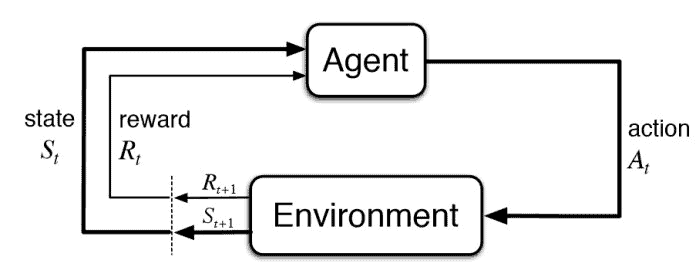 Reinforcement learning flow
RL is a type of machine learning that involves training agents to make a sequence of decisions in an environment in order to maximize a reward. The agent receives feedback in the form of rewards or punishments for its actions. Finally, the agent uses this feedback to learn what actions are most likely to lead to the greatest reward.
Feel free to check out this great video, for a more thorough introduction to Reinforcement Learning.
The Bellman Equation
The Bellman equation is a fundamental concept in reinforcement learning (RL) and is at the heart of the Q-learning algorithm. It is used to determine the optimal action to take in a given state.
It states that the optimal action-value function at a given state is the maximum expected return starting from that state. In other words, the optimal value function is the sum of the following:
-
The immediate reward received for taking a particular action
-
The expected return of the next action, discounted by a factor of gamma (γ). This discount factor represents the importance of future rewards (0 => only immediate rewards matter and 1 => all future rewards are equally important).
The Bellman equation can be expressed mathematically as follows:
 Bellman Equation for q* value
where
-
q(s, a)is the optimal action-value function -
Edenotes the word “expectation”, meaning we don’t know for sure that the equation is satisfied -
ris the reward received for taking actionain states -
γis the discount factor -
St+1 is the next state
-
a'is the next action.
The Bellman equation is used in Q-learning to update the action-value function based on the reward received for the current action and the expected return of the next action. By maximizing the action-value function, the Q-learning algorithm can learn the actions that are most likely to lead to the highest cumulative reward.
Q-learning algorithm and How it Works
Q-learning is a type of reinforcement learning algorithm that is used to find the optimal policy for an agent to follow in a given environment. It does this by using a table called the “q-table” to store the expected reward for taking a specific action in a specific state.
The q-table is initially filled with zeros. As the agent interacts with the environment, it updates the values in the q-table based on the rewards it receives. The agent follows an exploration-exploitation trade-off, meaning it will try out new actions to see if they lead to a higher reward, while also relying on the values in the q-table to guide its actions toward the most promising options.
The Exploration-Exploitation Trade-off
The exploration-exploitation trade-off refers to the balance between exploring new options and exploiting known good options in order to maximize reward. An agent faces this trade-off when deciding which actions to take in a given environment. If the agent always chooses the action with the highest expected reward, it may miss out on the potential for even higher rewards from unexplored options. On the other hand, if the agent always explores new options, it may not make the most efficient use of its time and resources. The optimal balance between exploration and exploitation depends on the specific context and the agent’s goals.
To balance exploration and exploitation, Q-learning uses an exploration policy, such as an ε-greedy policy. An ε-greedy policy allows the agent to choose a random action with a small probability (ε) and the action with the highest expected return with a high probability (1-ε). Accordingly, the agent tries out new actions and explores the environment while also exploiting its current knowledge to maximize reward.
The Q-learning Algorithm
- The agent selects an action based on either of the following:
-
The current state and the values in the q-table
-
A randomly chosen action.
-
-
The agent takes the action and the environment responds with a reward and the next state
- The agent updates the q-value for the taken action based on the reward and the expected future rewards
- This is done according to the Bellman Equation that we discussed earlier.
- The process repeats from step 1
As the agent continues to interact with the environment, the values in the q-table become more accurate and the agent’s policy becomes more optimal.
Limitations of Q-learning
Q-learning is a powerful algorithm for reinforcement learning (RL), but it has its limitations and challenges. Here are some of the key limitations and challenges of using Q-learning:
-
Data requirements: Q-learning requires a large amount of data to learn an accurate action-value function. This can be a challenge in real-world environments where it is difficult to collect a sufficient amount of data.
-
Convergence issues: Q-learning can sometimes have difficulty converging to the optimal action-value function, especially in environments with a large state space or a continuous action space. This can lead to suboptimal performance or even divergence of the algorithm.
-
Function approximation: In environments with a large state space, it can be impractical to learn an action-value function for every possible state.
-
Online learning: Q-learning is an online learning algorithm, which means that it updates the action-value function as it interacts with the environment. This can be a challenge in environments where the agent may need to wait a long time to receive a reward and update its action-value function.
-
Stochastic environments: In stochastic environments, the state transitions and reward distributions are not deterministic. This can make it difficult for Q-learning to learn the optimal action-value function.
Implementation
This implementation of Q-learning uses the OpenAI Gym library to create a simple environment called “FrozenLake-v0”, which consists of a 4x4 grid of blocks. The goal of the agent is to navigate from the start block to the goal block by taking actions to move left, right, up, or down. The environment provides observations, rewards, and whether the episode is done to the agent at each step.

Frozen Lake OpenAI Gym
The Code
import gym  # import the OpenAI Gym library
import numpy as np  # import NumPy library

# Create the environment
env = gym.make('FrozenLake-v1', is_slippery=False)

# Set parameters
alpha = 0.1  # learning rate
gamma = 0.6  # discount factor

# Set the action and state space sizes
n_actions = env.action_space.n
n_states = env.observation_space.n

# Initialize Q-table with zeros
Q = np.zeros((n_states, n_actions))

# Set number of episodes
num_episodes = 10000

# Create a list to store rewards
r_list = []

# Loop through episodes
for i in range(num_episodes):
    # Reset the environment and get the initial state
    state = env.reset()[0]
    r_all = 0
    done = False

    # The Q-Table learning algorithm
    while not done:
        # Choose an action by greedily (with noise) picking from Q table
        action = np.argmax(Q[state,:] + np.random.randn(1, n_actions) / (i+1))

        # Get new state and reward from environment
        new_state, reward, done, _, _ = env.step(action)

        # Update Q-Table with new knowledge
        Q[state, action] = Q[state, action] + alpha * (reward + gamma * np.max(Q[new_state, :]) - Q[state, action])

        # Update total reward
        r_all += reward

        # Set new state
        state = new_state

    # Append total reward for this episode to the reward list
    r_list.append(r_all)

print("Score over time: " +  str(sum(r_list)/num_episodes))
print("Final Q-Table Values")
print(Q)
Quick Explanation
The Q-learning algorithm is implemented using a loop that runs for a specified number of episodes. In each episode, the environment is reset and the agent chooses an action using the Q-table and an epsilon-greedy-equivalent policy.
Essentially, we add noise to the action selection. We also scale the values given to each action as time progresses. Therefore, with time, the algorithm becomes more and more deterministic, similar to epsilon-greedy.
Simulating the Policy
You can try running the calculated Q-table using the following code. You can copy-paste below the previous code to view the result at the end of the training:
# ---------- Simulate the policy ----------
policy = {}
for i, act in enumerate(np.argmax(Q, axis=1)):
    policy[i] = act

print("Policy:", policy)

path = []
dirs = ['left', 'down', 'right', 'up']

state = env.reset()[0]
r_all = 0
done = False
while not done:
    # Choose an action by greedily (with noise) picking from Q table
    action = np.argmax(Q[state,:])
    path.append(dirs[action])

    # Get new state and reward from environment
    new_state, reward, done, _, _ = env.step(action)

    # Update total reward
    r_all += reward

    # Set new state
    state = new_state

print("Path:", path)
print("Reward:", reward)
Final Thoughts
That’s it! Hope you found this post on Q-learning helpful. Q-learning was the basis for many powerful reinforcement learning algorithms. So, it’s good to have a basic idea about how it works. We’ll discuss more such RL algorithms, moving forward. In the meantime, feel free to check out some of my other RL-related posts here.